
Computing DSGE Models with
Recursive Preferences and Stochastic Volatility*
Keywords: DSGE models, recursive preferences, perturbation.
JEL Classification: C63, C68, E32.
1 Introduction
This paper compares different solution methods for computing the equilibrium of dynamic stochastic general equilibrium (DSGE) models with recursive preferences and stochastic volatility (SV). Both features have become very popular in finance and in macroeconomics as modelling devices to account for business cycle fluctuations and asset pricing. Recursive preferences, as those first proposed by Kreps and Porteus (1978) and later generalized by Epstein and Zin (1989 and 1991) and Weil (1990), are attractive for two reasons. First, they allow us to separate risk aversion and intertemporal elasticity of substitution (EIS). Second, they offer the intuitive appeal of having preferences for early or later resolution of uncertainty (see the reviews by Backus et al., 2004 and 2007, and Hansen et al. , 2007, for further details and references). SV generates heteroskedastic aggregate fluctuations, a basic property of many time series such as output (see the review by Fernandez-Villaverde and Rubio-Ramirez, 2010), and adds extra flexibility in accounting for asset pricing patterns. In fact, in an influential paper, Bansal and Yaron (2004) have argued that the combination of recursive preferences and SV is the key for their proposed mechanism, long-run risk, to be successful at explaining asset pricing.
But despite the popularity and importance of these issues, nearly nothing is known about the numerical properties of the different solution methods that solve equilibrium models with recursive preferences and SV. For example, we do not know how well value function iteration (VFI) performs or how good local approximations are compared with global ones. Similarly, if we want to estimate the model, we need to assess which solution method is sufficiently reliable yet quick enough to make the exercise feasible. More important, the most common solution algorithm in the DSGE literature, (log-) linearization, cannot be applied, since it makes us miss the whole point of recursive preferences or SV: the resulting (log-) linear decision rules are certainty equivalent and do not depend on risk aversion or volatility. This paper attempts to fill this gap in the literature, and therefore, it complements previous work by Aruoba et al. (2006), in which a similar exercise is performed with the neoclassical growth model with CRRA utility function and constant volatility.
We solve and simulate the model using four main approaches: perturbation (of second and third order), Chebyshev polynomials, and VFI. By doing so, we span most of the relevant methods in the literature. Our results provide a strong guess of how some other methods not covered here, such as finite elements, would work (rather similar to Chebyshev polynomials but more computationally intensive). We report results for a benchmark calibration of the model and for alternative calibrations that change the variance of the productivity shock, the risk aversion, and the intertemporal elasticity of substitution. In that way, we study the performance of the methods both for cases close to the CRRA utility function with constant volatility and for highly non-linear cases far away from the CRRA benchmark. For each method, we compute decision rules, the value function, the ergodic distribution of the economy, business cycle statistics, the welfare costs of aggregate fluctuations, and asset prices. Also, we evaluate the accuracy of the solution by reporting Euler equation errors.
We highlight four main results from our exercise. First, all methods provide a high degree of accuracy. Thus, researchers who stay within our set of solution algorithms can be confident that their quantitative answers are sound.
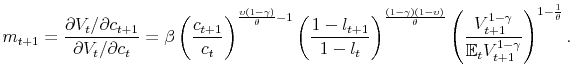
Second, perturbations deliver a surprisingly high level of accuracy with considerable speed. Both second- and third-order perturbations perform remarkably well in terms of accuracy for the benchmark calibration, being competitive with VFI or Chebyshev polynomials. For this calibration, a second-order perturbation that runs in a fraction of a second does nearly as well in terms of the average Euler equation error as a VFI that takes ten hours to run. Even in the extreme calibration with high risk aversion and high volatility of productivity shocks, perturbation works at a more than acceptable level. Since, in practice, perturbation methods are the only computationally feasible method to solve the medium-scale DSGE models used for policy analysis that have dozens of state variables (as in Smets and Wouters, 2007), this finding has an outmost applicability. Moreover, since implementing second- and third-order perturbations is feasible with off-the-shelf software like Dynare, which requires minimum programming knowledge by the user, our findings may induce many researchers to explore recursive preferences and/or SV in further detail. Two final advantages of perturbation are that, often, the perturbed solution provides insights about the economics of the problem and that it might be an excellent initial guess for VFI or for Chebyshev polynomials.
Third, Chebyshev polynomials provide a terrific level of accuracy with reasonable computational burden. When accuracy is most required and the dimensionality of the state space is not too high, as in our model, they are the obvious choice.
Fourth, we were disappointed by the poor performance of VFI, which, compared with Chebyshev, could not achieve a high accuracy even with a large grid. This suggests that we should relegate VFI to solving those problems where non-differentiabilities complicate the application of the previous methods.
The rest of the paper is organized as follows. In section 2, we present our test model. Section 3 describes the different solution methods used to approximate the decision rules of the model. Section 4 discusses the calibration of the model. Section 5 reports numerical results and section 6 concludes. An appendix provides some additional details.
2 The Stochastic Neoclassical Growth Model with Recursive Preferences and SV
We use the stochastic neoclassical growth model with recursive preferences and SV in the process for technology as our test case. We select this model for three reasons. First, it is the workhorse of modern macroeconomics. Even more complicated New Keynesian models with real and nominal rigidities, such as those in Woodford (2003) or Christiano et al. (2005), are built around the core of the neoclassical growth model. Thus, any lesson learned with it is likely to have a wide applicability. Second, the model is, except for the form of the utility function and the process for SV, the same test case as in Aruoba et al. (2006). This provides us with a set of results to compare to our findings. Three, the introduction of recursive preferences and SV make the model both more non-linear (and hence, a challenge for different solution algorithms) and potentially more relevant for practical use. For example, and as mentioned in the introduction, Bansal and Yaron (2004) have emphasized the importance of the combination of recursive preferences and time-varying volatility to account for asset prices.
The description of the model is straightforward, and we just go through the details required to fix notation. There is a representative household that has preferences over streams of consumption, ![]() , and leisure,
, and leisure, ![]() , represented by a recursive function of the form:
, represented by a recursive function of the form:
![\displaystyle U_{t}=\max_{c_{t},l_{t}}\left[ \left( 1-\beta \right) \left( c_{t}^{\upsilon }\left( 1-l_{t}\right) ^{1-\upsilon }\right) ^{\frac{1-\gamma }{\theta } }+\beta \left( {\mathbb{E}}_{t}U_{t+1}^{1-\gamma }\right) ^{\frac{1}{\theta } }\right] ^{\frac{\theta }{1-\gamma }}](img3.gif)
The parameters in these preferences include
 |
where
The household's budget constraint is given by:
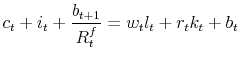 |
where
The final good in the economy is produced by a competitive firm with a Cobb-Douglas technology
![]() where
where ![]() is the productivity
level that follows:
is the productivity
level that follows:
Stationarity is the natural choice for our exercise. If we had a deterministic trend, we would only need to adjust
The innovation
![]() is scaled by a SV level
is scaled by a SV level
![]() which evolves as:
which evolves as:
where
The definition of equilibrium is standard and we skip it in the interest of space. Also, both welfare theorems hold, a fact that we will exploit by jumping back and forth between the solution of the social planner's problem and the competitive equilibrium. However, this is only to simplify our derivations. It is straightforward to adapt the solution methods described below to solve problems that are not Pareto optimal.
Thus, an alternative way to write this economy is to look at the value function representation of the social planner's problem in terms of its three state variables, capital ![]() ,
productivity
,
productivity ![]() , and volatility,
, and volatility,
![]() :
:
![\displaystyle V\left( k_{t},z_{t},\sigma _{t}\right) =\max_{c_{t},l_{t}}\left[ \left( 1-\beta \right) \left( c_{t}^{\upsilon }\left( 1-l_{t}\right) ^{1-\upsilon }\right) ^{\frac{1-\gamma }{\theta }}+\beta \left( {\mathbb{E}} _{t}V^{1-\gamma }\left( k_{t+1},z_{t+1},\sigma _{t+1}\right) \right) ^{\frac{ 1}{\theta }}\right] ^{\frac{\theta }{1-\gamma }}](img39.gif)
|
|
| s.t. |
|
Then, we can find the pricing kernel of the economy
 |
Now, note that:
 |
and:
|
where in the last step we use the result regarding
This equation shows how the pricing kernel is affected by the presence of recursive preferences. If
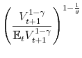
is equal to 1 and we get back the pricing kernel of the standard CRRA case. If
We identify the net return on equity with the marginal net return on investment:
with expected return
3 Solution Methods
We are interested in comparing different solution methods to approximate the dynamics of the previous model. Since the literature on computational methods is large, it would be cumbersome to review every proposed method. Instead, we select those methods that we find most promising.
Our first method is perturbation (introduced by Judd and Guu, 1992 and 1997 and nicely explained in Schmitt-Grohe and Uribe, 2004). Perturbation algorithms build a Taylor series expansion of the agents' decision rules. Often, perturbation methods are very fast and, despite their local nature, highly accurate in a large range of values of the state variables (Aruoba et al., 2006). This means that, in practice, perturbations are the only method that can handle models with dozens of state variables within any reasonable amount of time. Moreover, perturbation often provides insights into the structure of the solution and on the economics of the model. Finally, linearization and log-linearization, the most common solution methods for DSGE models, are particular cases of a perturbation of first order.
We implement a second- and a third-order perturbation of our model. A first-order perturbation is useless for our investigation: the resulting decision rules are certainty equivalent and, therefore, they depend on ![]() but not on
but not on ![]() or
or
![]() . In other words, the first-order decision rules of the model with recursive preferences coincide with the decision rules of the model with CRRA preferences with the same
. In other words, the first-order decision rules of the model with recursive preferences coincide with the decision rules of the model with CRRA preferences with the same
![]() and
and
![]() for any value of
for any value of ![]() or
or
![]() . We need to go, at least, to second-order decision rules to have terms that depend on
. We need to go, at least, to second-order decision rules to have terms that depend on ![]() or
or
![]() and, hence, allow recursive preferences or SV to play a role. Since the accuracy of second-order decision rules may not be high enough and, in addition, we want to explore
time-varying risk premia, we also compute a third-order perturbation. As we will document below, a third-order perturbation provides enough accuracy without unnecessary complications. Thus, we do not need to go to higher orders.
and, hence, allow recursive preferences or SV to play a role. Since the accuracy of second-order decision rules may not be high enough and, in addition, we want to explore
time-varying risk premia, we also compute a third-order perturbation. As we will document below, a third-order perturbation provides enough accuracy without unnecessary complications. Thus, we do not need to go to higher orders.
The second method is a projection algorithm with Chebyshev polynomials (Judd, 1992). Projection algorithms build approximated decision rules that minimize a residual function that measures the distance between the left- and right-hand side of the equilibrium conditions of the model. Projection methods are attractive because they offer a global solution over the whole range of the state space. Their main drawback is that they suffer from an acute curse of dimensionality that makes it challenging to extend it to models with many state variables. Among the many different types of projection methods, Aruoba et al. (2006) show that Chebyshev polynomials are particularly efficient. Other projection methods, such as finite elements or parameterized expectations, tend to perform somewhat worse than Chebyshev polynomials, and therefore, in the interest of space, we do not consider them.
Finally, we compute the model using VFI (Epstein and Zin, 1989, show that a version of the contraction mapping theorem holds in the value function of the problem with recursive preferences). VFI is slow and it suffers as well from the curse of dimensionality, but it is safe, reliable, and well understood. Thus, it is a natural default algorithm for the solution of DSGE models.
3.1 Perturbation
We describe now each of the different methods in more detail. We start by explaining how to use a perturbation approach to solve DSGE models using the value function of the household. We are not the first to explore the perturbation of value function problems. Judd (1998) already presents the idea of perturbing the value function instead of the equilibrium conditions of a model. Unfortunately, he does not elaborate much on the topic. Schmitt-Grohe and Uribe (2005) employ a perturbation approach to find a second-order approximation to the value function that allows them to rank different fiscal and monetary policies in terms of welfare. However, we follow Binsbergen et al. (2009) in their emphasis on the generality of the approach.1
To illustrate the procedure, we limit our exposition to deriving the second-order approximation to the value function and the decision rules of the agents. Higher-order terms are derived analogously, but the algebra becomes too cumbersome to be developed explicitly (in our application, the symbolic algebra is undertaken by Mathematica, which automatically generates Fortran 95 code that we can evaluate numerically). Hopefully, our steps will be enough to allow the reader to understand the main thrust of the procedure and obtain higher-order approximations by herself.
First, we rewrite the exogenous processes in terms of a perturbation parameter ![]() ,
,
When
Second, we note that, under differentiability assumptions, the second-order Taylor approximation of the value function around
![]() (the vectorial zero) is:
(the vectorial zero) is:
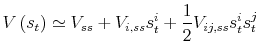 |
where:
- Each term
 is a scalar equal to a derivative of the value function evaluated at
 :
:
 for
for
 and
and
 for
for
- We use the tensors
 and
and
 , which eliminate the symbol
 when no confusion arises.
We can extend this notation to higher-order derivatives of the value function. This expansion could also be performed around a different point of the state space, such as the mode of the ergodic distribution of the state variables. In section 5, we discuss this point further.
Fernandez-Villaverde et al. (2010) show that many of these terms
![]() are zero (for instance, those implied by certainty equivalence in the first-order component). More directly related to this paper, Binsbergen et al. (2009) demonstrate that
are zero (for instance, those implied by certainty equivalence in the first-order component). More directly related to this paper, Binsbergen et al. (2009) demonstrate that
![]() does not affect the values of any of the coefficients except
does not affect the values of any of the coefficients except ![]() and
also that
and
also that
![]() . This result is intuitive, since the value function of a risk-averse agent is in general affected by uncertainty and we want to have an approximation with terms that capture
this effect and allow for the appropriate welfare ranking of decision rules. Indeed,
. This result is intuitive, since the value function of a risk-averse agent is in general affected by uncertainty and we want to have an approximation with terms that capture
this effect and allow for the appropriate welfare ranking of decision rules. Indeed, ![]() has a straightforward interpretation. At the deterministic steady state with
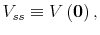
has a straightforward interpretation. At the deterministic steady state with ![]() (that is, even if we are in the stochastic economy, we just happen to be exactly at the steady state values of all the other states), we have:
(that is, even if we are in the stochastic economy, we just happen to be exactly at the steady state values of all the other states), we have:
 |
Hence
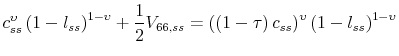
This cost of the business cycle can easily be transformed into consumption equivalent units. We can compute the percentage decrease in consumption ![]() that will make the household
indifferent between consuming
that will make the household
indifferent between consuming
![]() units per period with certainty or
units per period with certainty or ![]() units with
uncertainty. To do so, note that the steady-state value function is just
units with
uncertainty. To do so, note that the steady-state value function is just
![]() which implies that:
which implies that:
 |
or:
 |
Then:
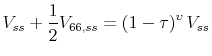
![\displaystyle \tau =1-\left[ 1+\frac{1}{2}\frac{V_{66,ss}}{V_{ss}}\right] ^{\frac{1}{ \upsilon }}.](img96.gif) |
We are perturbing the value function in levels of the variables. However, there is nothing special about levels and we could have done the same in logs (a common practice when linearizing DSGE models) or in any other function of the states. These changes of variables may improve the performance of perturbation (Fernández-Villaverde and Rubio-Ramí rez, 2006). By doing the perturbation in levels, we are picking the most conservative case for perturbation. Since one of the conclusions that we will reach from our numerical results is that perturbation works surprisingly well in terms of accuracy, that conclusion will only be reinforced by an appropriate change of variables.2
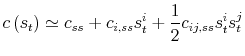
The decision rules can be expanded in the same way. For example, the second-order approximation of the decision rule for consumption is, under differentiability assumptions:
 |
where we have followed the same derivative and tensor notation as before.
As with the approximation of the value function, Binsbergen et al. (2009) show that ![]() does not affect the values of any of the coefficients except
does not affect the values of any of the coefficients except ![]() . This term is a constant that captures precautionary behavior caused by risk. This observation tells us two facts. First, a linear approximation to the decision rule does not depend on
. This term is a constant that captures precautionary behavior caused by risk. This observation tells us two facts. First, a linear approximation to the decision rule does not depend on ![]() (it is certainty equivalent), and therefore, if we are interested in recursive preferences, we need to go at least to a second-order approximation. Second, given some fixed parameter values, the difference between
the second-order approximation to the decision rules of a model with CRRA preferences and a model with recursive preferences is a constant. This constant generates a second, indirect effect, because it changes the ergodic distribution of the state variables and, hence, the points where we evaluate
the decision rules along the equilibrium path. These arguments demonstrate how perturbation methods can provide analytic insights beyond computational advantages and help in understanding the numerical results in Tallarini (2000). In the third-order approximation, all of the terms on functions of
(it is certainty equivalent), and therefore, if we are interested in recursive preferences, we need to go at least to a second-order approximation. Second, given some fixed parameter values, the difference between
the second-order approximation to the decision rules of a model with CRRA preferences and a model with recursive preferences is a constant. This constant generates a second, indirect effect, because it changes the ergodic distribution of the state variables and, hence, the points where we evaluate
the decision rules along the equilibrium path. These arguments demonstrate how perturbation methods can provide analytic insights beyond computational advantages and help in understanding the numerical results in Tallarini (2000). In the third-order approximation, all of the terms on functions of
![]() depend on
depend on ![]() .
.
Following the same steps, we can derive the decision rules for labor, investment, and capital. In addition we have functions that give us the evolution of other variables of interest, such as the pricing kernel or the risk-free gross interest rate ![]() . All of these functions have the same structure and properties regarding
. All of these functions have the same structure and properties regarding ![]() as the decision rule for consumption. In
the case of functions pricing assets, the second-order approximation generates a constant risk premium, while the third-order approximation creates a time-varying risk premium.
as the decision rule for consumption. In
the case of functions pricing assets, the second-order approximation generates a constant risk premium, while the third-order approximation creates a time-varying risk premium.
Once we have reached this point, there are two paths we can follow to solve for the coefficients of the perturbation. The first procedure is to write down the equilibrium conditions of the model plus the definition of the value function. Then, we take successive derivatives in this augmented set
of equilibrium conditions and solve for the unknown coefficients. This approach, which we call equilibrium conditions perturbation (ECP), gets us, after ![]() iterations, the
iterations, the ![]() -th-order approximation to the value function and to the decision rules.
-th-order approximation to the value function and to the decision rules.
A second procedure is to take derivatives of the value function with respect to states and controls and use those derivatives to find the unknown coefficient. This approach, which we call value function perturbation (VFP), delivers after
![]() steps, the
steps, the
![]() -th order approximation to the value function and the
-th order approximation to the value function and the ![]() th
order approximation to the decision rules.3 Loosely speaking, ECP undertakes the first step of VFP by hand by forcing the researcher to derive the equilibrium
conditions.
th
order approximation to the decision rules.3 Loosely speaking, ECP undertakes the first step of VFP by hand by forcing the researcher to derive the equilibrium
conditions.
The ECP approach is simpler but it relies on our ability to find equilibrium conditions that do not depend on derivatives of the value function. Otherwise, we need to modify the equilibrium conditions to include the definitions of the derivatives of the value function. Even if this is possible
to do (and not particularly difficult), it amounts to solving a problem that is equivalent to VFP. This observation is important because it is easy to postulate models that have equilibrium conditions where we cannot get rid of all the derivatives of the value function (for example, in problems of
optimal policy design). ECP is also faster from a computational perspective. However, VFP is only trivially more involved because finding the
![]() -th-order approximation to the value function on top of the
-th-order approximation to the value function on top of the ![]() -th order approximation requires nearly no additional effort.
-th order approximation requires nearly no additional effort.
The algorithm presented here is based on the system of equilibrium equations derived using the ECP. In the appendix, we derive a system of equations using the VFP. We take the first-order conditions of the social planner. First, with respect to consumption today:
 |
where
Third, with respect to labor:
 |
Then, we have
Once we substitute for the pricing kernel, the augmented equilibrium conditions are:
![\displaystyle V_{t}-\left[ \left( 1-\beta \right) \left( c_{t}^{\upsilon }\left( 1-l_{t}\right) ^{1-\upsilon }\right) ^{\frac{1-\gamma }{\theta }}+\beta \left( {\mathbb{E}}_{t}V^{1-\gamma }\left( k_{t+1},z_{t+1}\right) \right) ^{ \frac{1}{\theta }}\right] ^{\frac{\theta }{1-\gamma }}=0](img109.gif) |
|
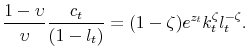
![\displaystyle \mathbb{E}_{t}\left[ \beta \left( \frac{c_{t+1}}{c_{t}}\right) ^{\frac{ 1-\gamma }{\theta }-1}\left( \frac{V_{t+1}^{1-\gamma }}{\mathbb{E} _{t}V_{t+1}^{1-\gamma }}\right) ^{1-\frac{1}{\theta }}\left( \zeta e^{z_{t+1}}k_{t+1}^{\zeta -1}l_{t+1}^{1-\zeta }+1-\delta \right) \right] -1=0](img110.gif)
|
|
 |
|
 |
|
plus the law of motion for productivity and volatility. Note that all the endogenous variables are functions of the states and that we drop the max operator in front of the value function because we are already evaluating it at the optimum. Thus, a more compact notation for the previous equilibrium conditions as a function of the states is:
where
In steady state,
![]() and the set of equilibrium conditions simplifies to:
and the set of equilibrium conditions simplifies to:
 |
|
a system of 6 equations on 6 unknowns,
To find the first-order approximation to the value function and the decision rules, we take first derivatives of the function ![]() with respect to the states
with respect to the states ![]() and evaluate them at
and evaluate them at
![]() :
:
This step gives us 48 different first derivatives (8 equilibrium conditions times the 6 variables of
To find the second-order approximation, we take derivatives on the first derivatives of the function ![]() , again with respect to the states and the perturbation parameter:
, again with respect to the states and the perturbation parameter:
This step gives us a new system of equations. Then, we plug in the terms that we already know from the steady state and from the first-order approximation and we get that the only unknowns left are the second-order terms of the value function and other functions of interest. Quite conveniently, this system of equations is linear and it can be solved quickly. Repeating these steps (taking higher-order derivatives, plugging in the terms already known, and solving for the remaining unknowns), we can get any arbitrary order approximation. For simplicity, and since we checked that we were already obtaining a high accuracy, we decided to stop at a third-order approximation (we are particularly interested in applying the perturbation for estimation purposes and we want to document how a third-order approximation is accurate enough for many problems without spending too much time deriving higher-order terms).
3.2 Projection
Projection methods take basis functions to build an approximated value function and decision rules that minimize a residual function defined by the augmented equilibrium conditions of the model. There are two popular methods for choosing basis functions: finite elements and the spectral method. We will present only the spectral method for several reasons: first, in the neoclassical growth model the decision rules and value function are smooth and spectral methods provide an excellent approximation. Second, spectral methods allow us to use a large number of basis functions, with the consequent high accuracy. Third, spectral methods are easier to implement. Their main drawback is that since they approximate the solution with a spectral basis, if the decision rules display a rapidly changing local behavior or kinks, it may be difficult for this scheme to capture those local properties.
Our target is to solve the decision rule for labor and the value function
![]() from:
from:
![\displaystyle \mathcal{H}(l_{t},V_{t})=\left[ \begin{array}{c} u_{c,t}-\beta \left( \mathbb{E}_{t}V_{t+1}^{1-\gamma }\right) ^{\frac{1}{ \theta }-1}\mathbb{E}_{t}\left[ V_{t+1}^{\frac{\left( 1-\gamma \right) \left( \theta -1\right) }{\theta }}u_{c,t+1}\left( \zeta e^{z_{t+1}}k_{t+1}^{\zeta -1}l_{t+1}^{1-\zeta }+1-\delta \right) \right] \\ V_{t}-\left[ (1-\beta )(c_{t}^{\upsilon }(1-l_{t}^{\upsilon }))^{\frac{ 1-\gamma }{\theta }}+\beta \mathbb{E}_{t}(V_{t+1}^{1-\gamma })^{\frac{1}{ \theta }}\right] ^{\frac{\theta }{1-\gamma }} \end{array} \right] =\mathbf{0}](img142.gif)
|
where, to save on notation, we define
 |
Then, from the static condition
and the resource constraint, we can find
Spectral methods solve this problem by specifying the decision rule for labor and the value function
![]() as linear combinations of weighted basis functions:
as linear combinations of weighted basis functions:
where
A common choice for the basis functions are Chebyshev polynomials because of their flexibility and convenience. Since their domain is [-1,1], we need to bound capital to the set [
![]() ], where
], where
![]() (
(
![]() ) is chosen sufficiently low (high) to bind only with extremely low probability, and define a linear map from those bounds into [-1,1]. Then, we set
) is chosen sufficiently low (high) to bind only with extremely low probability, and define a linear map from those bounds into [-1,1]. Then, we set
![]() where
where
![]() are Chebyshev polynomials and
are Chebyshev polynomials and
![]() is the linear mapping from [
is the linear mapping from [
![]() ] to [-1,1].
] to [-1,1].
By plugging
![]() and
and
![]() into
into
![]() , we find the residual function:
, we find the residual function:
We determine the coefficients
on
3.3 Value Function Iteration
Our final solution method is VFI. Since the dynamic algorithm is well known, our presentation is most brief. Consider the following Bellman operator:
![\displaystyle TV\left( k_{t},z_{t},\sigma _{t}\right) =\max_{c_{t},l_{t}}\left[ \left( 1-\beta \right) \left( c_{t}^{\upsilon }\left( 1-l_{t}\right) ^{1-\upsilon }\right) ^{\frac{1-\gamma }{\theta }}+\beta \left( {\mathbb{E}} _{t}V^{1-\gamma }\left( k_{t+1},z_{t+1},\sigma _{t+1}\right) \right) ^{\frac{ 1}{\theta }}\right] ^{\frac{\theta }{1-\gamma }}](img187.gif)
|
|
| s.t. |
|
To solve for this Bellman operator, we define a grid on capital,
- Set
 and
and
 for all
 and all
 .
. - For every
 use the Newton method to find
 ,
,
 ,
,
 that solve:
![\displaystyle \left( 1-\beta \right) \upsilon \frac{\left( c_{t}^{\upsilon }\left( 1-l_{t}\right) ^{1-\upsilon }\right) ^{\frac{1-\gamma }{\theta }}}{c_{t}} =\beta \left( \mathbb{E}_{t}\left( V_{t+1}^{n}\right) ^{1-\gamma }\right) ^{ \frac{1}{\theta }-1}\mathbb{E}_{t}\left[ \left( V_{t+1}^{n}\right) ^{-\gamma }V_{1,t+1}^{n}\right]](img197.gif)
- Construct
 from the Bellman equation:

- If
 , then
  and
go to 2. Otherwise, stop.
and
go to 2. Otherwise, stop.
To accelerate convergence and give VFI a fair chance, we implement a multigrid scheme as described by Chow and Tsitsiklis (1991). We start by iterating on a small grid. Then, after convergence, we add more points to the grid and recompute the Bellman operator using the previously found value function as an initial guess (with linear interpolation to fill the unknown values in the new grid points). Since the previous value function is an excellent grid, we quickly converge in the new grid. Repeating these steps several times, we move from an initial 23,000-point grid into a final one with 375,000 points (3,000 points for capital, 25 for productivity, and 5 for volatility).
4 Calibration
We now select a benchmark calibration for our numerical computations. We follow the literature as closely as possible and select parameter values to match, in the steady state, some basic observations of the U.S. economy (as we will see below, for the benchmark calibration, the means of the
ergodic distribution and the steady-state values are nearly identical). We set the discount factor
![]() to generate an annual interest rate of around 3.6 percent. We set the parameter that governs labor supply,
to generate an annual interest rate of around 3.6 percent. We set the parameter that governs labor supply, ![]()
![]() , to get the representative household to work one-third of its time. The elasticity of output to capital,
, to get the representative household to work one-third of its time. The elasticity of output to capital, ![]()
![]() matches the labor share of national income. A value of the depreciation rate
matches the labor share of national income. A value of the depreciation rate
![]() matches the ratio of investment-output. Finally,
matches the ratio of investment-output. Finally,
![]() and
and
![]() are standard values for the stochastic properties of the Solow residual. For the SV process, we pick
are standard values for the stochastic properties of the Solow residual. For the SV process, we pick ![]() and
and
![]() to match the persistence and standard deviation of the heteroskedastic component of the Solow residual during the last 5 decades.
to match the persistence and standard deviation of the heteroskedastic component of the Solow residual during the last 5 decades.
Since we want to explore the dynamics of the model for a range of values that encompasses all the estimates from the literature, we select four values for the parameter that controls risk aversion, ![]() , 2, 5, 10, and 40, and two values for EIS
, 2, 5, 10, and 40, and two values for EIS ![]() , 0.5, and 1.5, which bracket most of the values used in the literature (although many authors prefer smaller values for
, 0.5, and 1.5, which bracket most of the values used in the literature (although many authors prefer smaller values for
![]() , we found that the simulation results for smaller
, we found that the simulation results for smaller ![]() 's do not change much
from the case when
's do not change much
from the case when ![]()
![]() ). We then compute the model for all eight combinations
of values of
). We then compute the model for all eight combinations
of values of ![]() and
and ![]() , that is
, that is
![]() ,
,
![]() ,
,
![]() , and so on. When
, and so on. When ![]()
![]() and
and ![]() , we are back in the standard CRRA case. However, in the interest of space, we will report only a
limited subset of results that we find are the most interesting ones.
, we are back in the standard CRRA case. However, in the interest of space, we will report only a
limited subset of results that we find are the most interesting ones.
We pick as the benchmark case the calibration
![]() . These values reflect an EIS centered around the median of the estimates in the literature, a reasonably high level of
risk aversion, and the observed volatility of productivity shocks. To check robustness, we increase, in the extreme case, the risk aversion, the average standard deviation of the productivity shock, and the standard deviation of the innovations to volatility to
. These values reflect an EIS centered around the median of the estimates in the literature, a reasonably high level of
risk aversion, and the observed volatility of productivity shocks. To check robustness, we increase, in the extreme case, the risk aversion, the average standard deviation of the productivity shock, and the standard deviation of the innovations to volatility to
![]() . This case combines levels of risk aversion that are in the upper bound of all estimates in the literature with huge
productivity shocks. Therefore, it pushes all solution methods to their limits, in particular, making life hard for perturbation since the interaction of the large precautionary behavior induced by
. This case combines levels of risk aversion that are in the upper bound of all estimates in the literature with huge
productivity shocks. Therefore, it pushes all solution methods to their limits, in particular, making life hard for perturbation since the interaction of the large precautionary behavior induced by ![]() and large shocks will move the economy far away from the deterministic steady state. We leave the discussion of the effects of
and large shocks will move the economy far away from the deterministic steady state. We leave the discussion of the effects of ![]() for the robustness analysis at
the end of the next section.
for the robustness analysis at
the end of the next section.
5 Numerical Results
In this section we report our numerical findings. First, we present and discuss the computed decision rules. Second, we show the results of simulating the model. Third, we report the Euler equation errors. Fourth, we discuss the effects of changing the EIS and the perturbation point. Finally, we discuss implementation and computing time.
5.1 Decision Rules
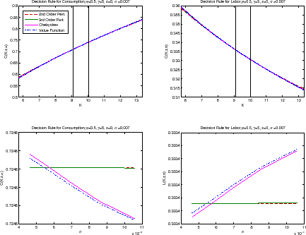
Figure 1 plots the decision rules of the household for consumption and labor in the benchmark case. In the top two panels, we plot the decision rules along the capital axis when ![]() and
and
![]() . The capital interval is centered on the steady-state level of capital of 9.54 with a width of
. The capital interval is centered on the steady-state level of capital of 9.54 with a width of ![]() [5.72,13.36]. This interval is big enough to encompass all the simulations. We also plot, with two vertical lines, the 10 and 90 percentile of the ergodic distribution of capital.4 Since all methods provide nearly indistinguishable answers, we observe only one line in both panels. It is possible to appreciate miniscule differences in labor supply between second-order perturbation and the other
methods only when capital is far from its steady-state level. Monotonicity of the decision rules is preserved by all methods.5 We must be cautious, however,
mapping differences in choices into differences in utility. The Euler error function below provides a better view of the welfare consequences of different approximations.
[5.72,13.36]. This interval is big enough to encompass all the simulations. We also plot, with two vertical lines, the 10 and 90 percentile of the ergodic distribution of capital.4 Since all methods provide nearly indistinguishable answers, we observe only one line in both panels. It is possible to appreciate miniscule differences in labor supply between second-order perturbation and the other
methods only when capital is far from its steady-state level. Monotonicity of the decision rules is preserved by all methods.5 We must be cautious, however,
mapping differences in choices into differences in utility. The Euler error function below provides a better view of the welfare consequences of different approximations.
In the bottom two panels, we plot the decision rules as a function of
![]() when
when
![]() and
and ![]() Both VFI and Chebyshev polynomials capture well
precautionary behavior: the household consumes less and work more when
Both VFI and Chebyshev polynomials capture well
precautionary behavior: the household consumes less and work more when
![]() is higher. In comparison, it would seem that perturbations do a much poorer job at capturing this behavior. However, this is not the right interpretation. In a second-order
perturbation, the effect of
is higher. In comparison, it would seem that perturbations do a much poorer job at capturing this behavior. However, this is not the right interpretation. In a second-order
perturbation, the effect of
![]() only appears in a term where
only appears in a term where
![]() interacts with
interacts with ![]() . Since here we are plotting a cut of the decision
rule while keeping
. Since here we are plotting a cut of the decision
rule while keeping ![]() , that term drops out and the decision rule that comes from a second-order approximation is a flat line. In the third-order perturbation,
, that term drops out and the decision rule that comes from a second-order approximation is a flat line. In the third-order perturbation,
![]() appears by itself, but raised to its cube. Hence, the slope of the decision rule is negligible. As we will see below, the interaction effects of
appears by itself, but raised to its cube. Hence, the slope of the decision rule is negligible. As we will see below, the interaction effects of
![]() with other variables, which are hard to visualize in two-dimensional graph, are all that we need to deliver a satisfactory overall performance.
with other variables, which are hard to visualize in two-dimensional graph, are all that we need to deliver a satisfactory overall performance.
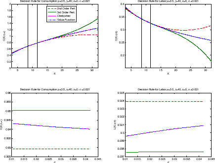
We see bigger differences in the decision rules as we increase the risk aversion and the variance of innovations. Figure 2 plots the decision rules for the extreme calibration following the same convention than before. In this figure, we change the capital interval where we compute the top decision rules to [3,32] (roughly 1/3 and 3 times the steady-state capital) because, owing to the high variance of the calibration, the equilibrium paths fluctuate through much wider ranges of capital.
We highlight several results. First, all the methods deliver similar results in our original capital interval for the benchmark calibration. Second, as we go far away from the steady state, VFI and the Chebyshev polynomial still overlap with each other (and, as shown by our Euler error computations below, we can roughly take them as the "exact" solution), but second- and third-order approximations start to deviate. Third, the decision rule for consumption approximated by the third-order perturbation changes from concavity into convexity for values of capital bigger than 15. This phenomenon (also documented in Aruoba et al. 2006) is due to the poor performance of local approximation when we move too far away from the expansion point and the polynomials begin to behave wildly. Numerically, this issue is irrelevant because the problematic region is visited with nearly zero probability.
5.2 Simulations
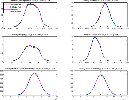
Applied economists often characterize the behavior of the model through statistics from simulated paths of the economy. We simulate the model, starting from the deterministic steady state, for 10,000 periods, using the decision rules for each of the eight combinations of risk aversion and EIS discussed above. To make the comparison meaningful, the shocks are common across all paths. We discard the first 1,000 periods as a burn-in to eliminate the transition from the deterministic steady state of the model to the middle regions of the ergodic distribution of capital. This is usually achieved in many fewer periods than the ones in our burn-in, but we want to be conservative in our results. The remaining observations constitute a sample from the ergodic distribution of the economy.
For the benchmark calibration, the simulations from all of the solution methods generate almost identical equilibrium paths (and therefore we do not report them). We focus instead on the densities of the endogenous variables as shown in figure 3 (remember that volatility and productivity are identical across the different solution methods). Given the low risk aversion and SV of the productivity shocks, all densities are roughly centered around the deterministic steady-state value of the variable. For example, the mean of the distribution of capital is only 0.2 percent higher than the deterministic value. Also, capital is nearly always between 8.5 and 10.5. This range will be important below to judge the accuracy of our approximations.
Table 2 reports business cycle statistics and, because DSGE models with recursive preferences and SV are often used for asset pricing, the average and variance of the (quarterly) risk-free rate and return on capital. Again, we see that nearly all values are the same, a simple consequence of the similarity of the decision rules.
The welfare cost of the business cycle is reported in table 3 in consumption equivalent terms. The computed costs are actually negative. Besides the Jensen's effect on average productivity, this is also due to the fact that when we have leisure in the utility function, the indirect utility function may be convex in input prices (agents change their behavior over time by a large amount to take advantage of changing productivity). Cho and Cooley (2000) present a similar example. Welfare costs are comparable across methods. Remember that the welfare cost of the business cycle for the second- and third-order perturbations is the same because the third-order terms all drop or are zero when evaluated at the steady state.
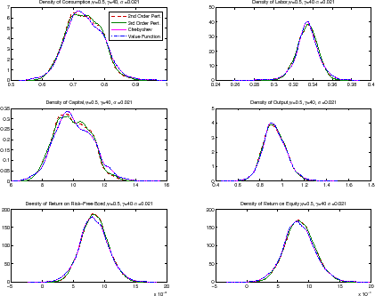
When we move to the extreme calibration, we see more differences. Figure 4 plots the histograms of the simulated series for each solution method. Looking at quantities, the histograms of consumption, output, and labor are the same across all of the methods. The ergodic distribution of capital puts nearly all the mass between values of 6 and 15. This considerable move to the right in comparison with figure 3 is due to the effect of precautionary behavior in the presence of high risk aversion, large productivity shocks, and high SV. Capital also visits low values of capital more than in the benchmark calibration because of large, persistent productivity shocks. In any case, the translation is more pronounced to the right than to the left.
Table 4 reports business cycle statistics. Differences across methods are minor in terms of means (note that the mean of the risk-free rate is lower than in the benchmark calibration because of the extra accumulation of capital induced by precautionary behavior). In terms of variances, the second-order perturbation produces less volatility than all other methods. This suggests that a second-order perturbation may not be good enough if we face high variance of the shocks and/or high risk aversion. A third-order perturbation, in comparison, eliminates most of the differences and delivers nearly the same implications as Chebyshev polynomials or VFI.
Finally, table 5 presents the welfare cost of the business cycle. Now, in comparison with the benchmark calibration, the welfare cost of the business cycle is positive and significant, slightly above 1.1 percent. This is not a surprise, since we have both a large risk aversion and productivity shocks with an average standard deviation three times as big as the observed one. All methods deliver numbers that are close.
5.3 Euler Equation Errors
While the plots of the decision rules and the computation of densities and business cycle statistics that we presented in the previous subsection are highly informative, it is also important to evaluate the accuracy of each of the procedures. Euler equation errors, introduced by Judd (1992), have become a common tool for determining the quality of the solution method. The idea is to observe that, in our model, the intertemporal condition:
where
![\displaystyle EE^{i}\left( k_{t},z_{t},\sigma _{t}\right) =1-\frac{\left[ \frac{\beta ({ \mathbb{E}}_{t}\left( V_{t+1}^{i}\right) ^{1-\gamma })^{\frac{1}{\theta }-1}{ \mathbb{E}}_{t}\left( \left( V_{t+1}^{i}\right) ^{\frac{(\gamma -1)(1-\theta )}{\theta }}u_{c,t+1}^{i}R\left( k_{t},z_{t},\sigma _{t};z_{t+1},\sigma _{t+1}\right) \right) }{\frac{1-\gamma }{\theta }\upsilon (1-l_{t}^{i})^{\left( 1-\upsilon \right) \frac{1-\gamma }{\theta }}}\right] ^{\frac{1}{\upsilon \frac{1-\gamma }{\theta }-1}}}{c_{t}^{i}}](img232.gif)
|
This function determines the (unit free) error in the Euler equation as a fraction of the consumption given the current states and solution method
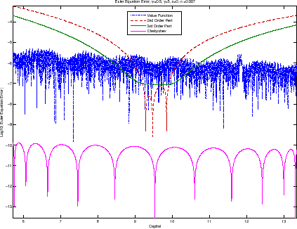
Figure 5 displays a transversal cut of the errors for the benchmark calibration when ![]() and
and
![]() . Other transversal cuts at different technology and volatility levels reveal similar patterns. The first lesson from figure 5 is that all methods deliver high
accuracy. We know from figure 3 that capital is nearly always between 8.5 and 10.5. In that range, the (log10) Euler equation errors are at most -5, and most of the time they are even smaller. For instance, the second- and third-order perturbations have an Euler equation error of around -7 in the
neighborhood of the deterministic steady state, VFI of around -6.5, and Chebyshev an impressive -11/-13. The second lesson from figure 5 is that, as expected, global methods (Chebyshev and VFI) perform very well in the whole range of capital values, while perturbations deteriorate as we move away
from the steady state. For second-order perturbation, the Euler error in the steady state is almost four orders of magnitude smaller than on the boundaries. Third-order perturbation is around half an order of magnitude more accurate than second-order perturbation over the whole range of values
(except in a small region close to the deterministic steady state).
. Other transversal cuts at different technology and volatility levels reveal similar patterns. The first lesson from figure 5 is that all methods deliver high
accuracy. We know from figure 3 that capital is nearly always between 8.5 and 10.5. In that range, the (log10) Euler equation errors are at most -5, and most of the time they are even smaller. For instance, the second- and third-order perturbations have an Euler equation error of around -7 in the
neighborhood of the deterministic steady state, VFI of around -6.5, and Chebyshev an impressive -11/-13. The second lesson from figure 5 is that, as expected, global methods (Chebyshev and VFI) perform very well in the whole range of capital values, while perturbations deteriorate as we move away
from the steady state. For second-order perturbation, the Euler error in the steady state is almost four orders of magnitude smaller than on the boundaries. Third-order perturbation is around half an order of magnitude more accurate than second-order perturbation over the whole range of values
(except in a small region close to the deterministic steady state).
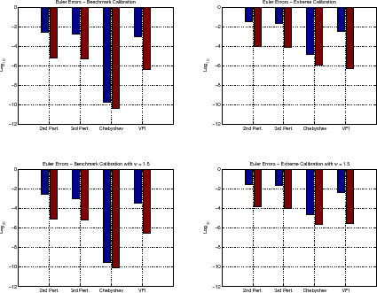
There are two complementary ways to summarize the information from Euler equation error functions. First, we report the maximum error in our interval (capital between 60 percent and 140 percent of the steady state and the grids for productivity and volatility). The maximum Euler error is useful because it bounds the mistake owing to the approximation. The second procedure for summarizing Euler equation errors is to integrate the function with respect to the ergodic distribution of capital and productivity to find the average error. We can think of this exercise as a generalization of the Den Haan-Marcet test (Den Haan and Marcet, 1994). The top- left panel in Figure 6 reports the maximum Euler error (darker bars) and the integral of the Euler error for the benchmark calibration. Both perturbations have a maximum Euler error of around -2.7, VFI of -3.1, and Chebyshev, an impressive -9.8. We read this result as indicating that all methods perform adequately. Both perturbations have roughly the same integral of the Euler error (around -5.3), VFI a slightly better -6.4, while Chebyshev polynomials do fantastically well at -10.4 (the average loss of welfare is $1 for each $500 billion). But even an approximation with an average error of $1 for each $200,000, such as the one implied by third-order perturbation, must suffice for most relevant applications.
We repeat our exercise for the extreme calibration. As we did when we computed the decision rules of the agents, we have changed the capital interval to [3,32]. The top-right panel in Figure 6 reports maximum Euler equation errors and their integrals. The maximum Euler equation error is large for perturbation methods while it is rather small using Chebyshev polynomials. However, given the very large range of capital used in the computation, this maximum Euler error provides a too negative view of accuracy. We find the integral of the Euler equation error to be more instructive. With a second-order perturbation, we have -4.02 and with a third-order perturbation we have -4.12. To evaluate this number, remember that we have extremely high risk aversion and large productivity shocks. Even in this challenging environment, perturbations deliver a high degree of accuracy. VFI does not display a big loss of precision compared to the benchmark case. On the other hand, Chebyshev polynomials deteriorate somewhat, but the accuracy it delivers it is still of $1 out of each $1 million spent.
5.4 Robustness: Changing the EIS and Changing the Perturbation Point
In the results we reported above, we kept the EIS equal to 0.5, a conventional value in the literature, while we modified the risk aversion and the volatility of productivity shocks. However, since some researchers prefer higher values of the EIS (see, for instance, Bansal and Yaron, 2004, a
paper that we have used to motivate our investigation), we also computed our model with ![]()
![]() . Basically our results were unchanged. To save on space, we concentrate only on the Euler equation errors (decision rules and simulation paths are available upon request). In the bottom-left panel in Figure 6, we report the maxima of the Euler equation errors and their integrals
with respect to the ergodic distribution. The relative size and values of the entries in this table are quite similar to the values reported for the benchmark calibration (except, partially, VFI that performs a bit better). The bottom-right panel in Figure 6 repeats the same exercise for the
extreme calibration. Again, the entries in the table are very close to the ones in the extreme calibration (and now, VFI does not perform better than when
. Basically our results were unchanged. To save on space, we concentrate only on the Euler equation errors (decision rules and simulation paths are available upon request). In the bottom-left panel in Figure 6, we report the maxima of the Euler equation errors and their integrals
with respect to the ergodic distribution. The relative size and values of the entries in this table are quite similar to the values reported for the benchmark calibration (except, partially, VFI that performs a bit better). The bottom-right panel in Figure 6 repeats the same exercise for the
extreme calibration. Again, the entries in the table are very close to the ones in the extreme calibration (and now, VFI does not perform better than when ![]()
![]() ).
).
As a final robustness test, we computed the perturbations not around the deterministic steady state (as we did in the main text), but around a point close to the mode of the ergodic distribution of capital. This strategy, if perhaps difficult to implement because of the need to compute the mode of the ergodic distribution,6 could deliver better accuracy because we approximate the value function and decision rules in a region where the model spends more time. As we suspected, we found only trivial improvements in terms of accuracy. Moreover, expanding at a point different from the deterministic steady state has the disadvantage that the theorems that ensure the convergence of the Taylor approximation might fail (see theorem 6 in Jin and Judd, 2002).
5.5 Implementation and Computing Time
We briefly discuss implementation and computing time. For the benchmark calibration, second-order perturbation and third- order perturbation algorithms take only 0.02 second and 0.05 second, respectively, in a 3.3GHz Intel PC with Windows 7 (the reference computer for all times below), and it is simple to implement: 664 lines of code in Fortran 95 for second order and 1133 lines of code for third order, plus in both cases, the analytical derivatives of the equilibrium conditions that Fortran 95 borrows from a code written in Mathematica 6.7 The code that generates the analytic derivatives has between 150 to 210 lines, although Mathematica is much less verbose. While the number of lines doubles in the third order, the complexity in terms of coding does not increase much: the extra lines are mainly from declaring external functions and reading and assigning values to the perturbation coefficients. An interesting observation is that we only need to take the analytic derivatives once, since they are expressed in terms of parameters and not in terms of parameter values. This allows Fortran to evaluate the analytic derivatives extremely fast for new combinations of parameter values. This advantage of perturbation is particularly relevant when we need to solve the model repeatedly for many different parameter values, for example, when we are estimating the model. For completeness, the second-order perturbation was also run in Dynare (although we had to use version 4.0, which computes analytic derivatives, instead of previous versions, which use numerical derivatives that are not accurate enough for perturbation). This run was a double-check of the code and a test of the feasibility of using off-the-shelf software to solve DSGE models with recursive preferences.
The projection algorithm takes around 300 seconds, but it requires a good initial guess for the solution of the system of equations. Finding the initial guess for some combination of parameter values proved to be challenging. The code is 652 lines of Fortran 95. Finally, the VFI code is 707 lines of Fortran 95, but it takes about ten hours to run.
6 Conclusions
In this paper, we have compared different solution methods for DSGE models with recursive preferences and SV. We evaluated the different algorithms based on accuracy, speed, and programming burden. We learned that all of the most promising methods (perturbation, projection, and VFI) do a fair job in terms of accuracy. We were surprised by how well simple second-order and third-order perturbations perform even for fairly non-linear problems. We were impressed by how accurate Chebyshev polynomials can be. However, their computational cost was higher and we are concerned about the curse of dimensionality. In any case, it seems clear to us that, when accuracy is the key consideration, Chebyshev polynomials are the way to go. Finally, we were disappointed by VFI since even with 125,000 points in the grid, it only did marginally better than perturbation and it performed much worse than Chebyshev polynomials in our benchmark calibration. This suggests that unless there are compelling reasons such as non-differentiabilities or non-convexities in the model, we better avoid VFI.
A theme we have not developed in this paper is the possibility of interplay among different solution methods. For instance, we can compute extremely easily a second-order approximation to the value function and use it as an initial guess for VFI. This second-order approximation is such a good guess that VFI will converge in few iterations. We verified this idea in non-reported experiments, where VFI took one-tenth of the time to converge once we used the second-order approximation to the value function as the initial guess. This approach may even work when the true value function is not differentiable at some points or has jumps, since the only goal of perturbation is to provide a good starting point, not a theoretically sound approximation. This algorithm may be particularly useful in problems with many state variables. More research on this type of hybrid method is a natural extension of our work.
We close the paper by pointing out that recursive preferences are only one example of a large class of non-standard preferences that have received much attention by theorists and applied researchers over the last several years (see Backus, Routledge, and Zin, 2004). Having fast and reliable solution methods for this class of new preferences will help researchers to sort out which of these preferences deserve further attention and to derive empirical implications. Thus, this paper is a first step in the task of learning how to compute DSGE models with non-standard preferences.
| Parameter |
|
|||||||
| Value | 0.991 | 0.357 | 0.3 | 0.0196 | 0.95 | 0.007 | 0.9 | 0.06 |
| Mean | |||||
| Second-Order Perturbation | 0.7253 | 0.9128 | 0.1873 | 0.9070 | 0.9078 |
| Third-Order Perturbation | 0.7257 | 0.9133 | 0.1875 | 0.9062 | 0.9069 |
| Chebyshev Polynomial | 0.7256 | 0.9130 | 0.1875 | 0.9063 | 0.9066 |
| Value Function Iteration | 0.7256 | 0.9130 | 0.1875 | 0.9063 | 0.9066 |
| Variance | |||||
| Second-Order Perturbation | 0.0331 | 0.1084 | 0.0293 | 0.0001 | 0.0001 |
| Third-Order Perturbation | 0.0330 | 0.1079 | 0.0288 | 0.0001 | 0.0001 |
| Chebyshev Polynomial | 0.0347 | 0.1117 | 0.0313 | 0.0001 | 0.0001 |
| Value Function Iteration | 0.0347 | 0.1117 | 0.0313 | 0.0001 | 0.0001 |
| 2nd-Order Pert. | 3rd-Order Pert. | Chebyshev | Value Function |
| -2.0864e(-5) | -2.0864e(-5) | -3.2849e(-5) | -3.2849e(-5) |
| Mean | |||||
| Second-Order Perturbation | 0.7338 | 0.9297 | 0.1950 | 0.8432 | 0.8562 |
| Third-Order Perturbation | 0.7344 | 0.9311 | 0.1955 | 0.8416 | 0.8529 |
| Chebyshev Polynomial | 0.7359 | 0.9329 | 0.1970 | 0.8331 | 0.8402 |
| Value Function Iteration | 0.7359 | 0.9329 | 0.1970 | 0.8352 | 0.8403 |
| Variance | |||||
| Second-Order Perturbation | 0.2956 | 1.0575 | 0.2718 | 0.0004 | 0.0004 |
| Third-Order Perturbation | 0.3634 | 1.2178 | 0.3113 | 0.0004 | 0.0005 |
| Chebyshev Polynomial | 0.3413 | 1.1523 | 0.3425 | 0.0005 | 0.0006 |
| Value Function Iteration | 0.3414 | 1.1528 | 0.3427 | 0.0005 | 0.0006 |
| 2nd-Order Pert. | 3rd-Order Pert. | Chebyshev | Value Function |
| 1.1278e-2 | 1.1278e-2 | 1.2855e-2 | 1.2838e-2 |
7 Appendix
In this appendix, we present the steady state of the model and the alternative perturbation approach, the value function perturbation (VFP).
7.1 Steady State of the Model
To solve the system:
 |
|
note first that:
 |
Now, from the leisure-consumption condition:
Then:
and:
 |
|
 |
from which we can find
7.2 Value Function Perturbation (VFP)
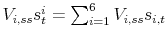
We mentioned in the main text that instead of perturbing the equilibrium conditions of the model, we could directly perturb the value function in what we called value function perturbation (VFP). To undertake the VFP, we write the value function as:
![\displaystyle V\left( k_{t},z_{t},\sigma _{t};\chi \right) =\max_{c_{t},l_{t}}\left[ \left( 1-\beta \right) \left( c_{t}^{\upsilon }\left( 1-l_{t}\right) ^{1-\upsilon }\right) ^{\frac{1-\gamma }{\theta }}+\beta {\mathbb{E}} _{t}V^{1-\gamma }\left( k_{t+1},z_{t+1},\sigma _{t+1};\chi \right) ^{\frac{1 }{\theta }}\right] ^{\frac{\theta }{1-\gamma }}](img256.gif)
|
To find a second-order approximation to the value function, we take derivatives of the value function with respect to controls (
![]() ), states (
), states (
![]() ), and the perturbation parameter
), and the perturbation parameter ![]() . We collect these 6
equations, together with the resource constraint, the value function itself, and the exogenous processes in a system:
. We collect these 6
equations, together with the resource constraint, the value function itself, and the exogenous processes in a system:
where the hat over
After solving for the steady state of this system, we take derivatives of the function
![]() with respect to
with respect to ![]() ,
, ![]() ,
,
![]() , and
, and ![]() :
:
and we solve for the unknown coefficients. This solution will give us a second-order approximation of the value function but only a first-order approximation of the decision rules. By repeating these steps