
The Influence of Fannie and Freddie on Mortgage Loan Terms
Keywords: Government-sponsored enterprises, mortgages.
Abstract:
This paper uses a novel instrumental variables approach to quantify the effect that GSE purchase eligibility had on equilibrium mortgage loan terms in the period from 2003 to 2007. The technique is designed to eliminate sources of bias that may have affected previous studies. GSE eligibility appears to have lowered interest rates by about 10 basis points, encouraged fixed-rate loans over ARMs, and discouraged low-documentation and brokered loans. There is no measurable effect on loan performance or on the prevalence of certain types of "exotic" mortgages. The overall picture suggests that GSE purchases had only a modest impact on loan terms during this period.
JEL Classification: G21, G28, H81, N22.
1 Introduction
In 2011 over 75% of all mortgages originated in the United States--over $1 trillion worth--passed through the hands of the Federal National Mortgage Association (Fannie Mae) and the Federal Home Loan Mortgage Corporation (Freddie Mac) (Inside Mortgage Finance, 2012). These institutions, known as the Government-Sponsored Enterprises (GSEs), have traditionally been private corporations with a public charter, operating with the implicit backing of the United States government.1 Their mission, as defined by their regulator the Federal Housing Finance Agency (FHFA), is to promote liquidity, affordability, and stability in the U.S. mortgage market. The GSEs are meant to accomplish these goals by purchasing mortgage loans on the secondary market, which they then package into securities or hold in portfolio. In September 2008 the GSEs' implicit government backing became explicit when, in the throes of the financial crisis and facing possible bankruptcy, both Fannie and Freddie were placed in conservatorship by FHFA. The cost to taxpayers of their bailout has been estimated at $317 billion so far (Congressional Budget Office, 2011).
Given the GSEs' vast scale, the liability they represent to taxpayers, and the decisions that must soon be made about their future, it is crucial to understand how exactly they affect the mortgage markets in which they operate. Unfortunately, modeling GSE activity and estimating its effect is a challenge. Fannie and Freddie are for-profit enterprises bound by a government-mandated mission that is likely at odds with their profit motive (Jaffee, 2009). As such, it is unclear what they maximize. Furthermore, they are large relative to the market. How they affect consumer outcomes, each other, and the rest of the market depends upon details of market structure. For instance, Passmore et al. (2002) show that whether or not lower capital costs (due to the implicit government subsidy) are ultimately passed on to borrowers in the form of lower mortgage rates depends crucially on the degree of competition or collusion between Fannie and Freddie, which is theoretically ambiguous.2 The GSEs' huge market share may also affect their behavior in other ways. Bubb & Kaufman (2009), for instance, explore how the GSEs' size may allow them to incentivize mortgage originators using a toolbox of strategies to that is unavailable to private-label securitizers.
Empirical estimation of the GSEs' impact on outcomes such as interest rates, default rates, and contract structures faces at least three important obstacles: selection bias, externalities, and sorting bias. First, in part due to their government mandate, the loans GSEs buy are not a random subset of all loans. GSE-purchased mortgage loans on average differ along several dimensions, including loan size and borrower creditworthiness, from loans purchased by private-label securitizers or left in the portfolio of originating lenders. Such selection must be separated from the true treatment effect of GSE purchases.
Second, even if GSE purchases were indeed random, it would not be sufficient to simply compare mortgages bought by the GSEs with those bought by private securitizers or left in portfolio. GSEs may affect the markets in which they operate by changing equilibrium prices and contract structures of all loans, not only those they buy. In other words, eligibility for GSE purchase may influence loan characteristics both for loans that are purchased and those that, despite being eligible, are not. Because of the potential for such pecuniary externalities, estimates based on comparing loans purchased by GSEs with loans not purchased will be biased toward zero, even when purchases are randomly assigned. In order to account for such externalities the ideal experiment is instead to compare loans in two similar markets, one in which the GSEs make purchases and one in which they do not, regardless of whether the individual loans being compared are ever bought by the GSEs.
Third, to the extent that GSE purchase eligibility may lead to loan terms that are more (or less) favorable to borrowers, potential borrowers may adjust their loan attributes in order to qualify for (or avoid) categories of loan that the GSEs are likely to buy. Such customer sorting is another potential source of bias. If borrowers sorting into GSE-eligible loans are different from other borrowers, and if those differences influence the features of the loans they receive--for instance, due to preferences or risk-based pricing--then customer sorting will bias estimates of GSE treatment effects.
To illustrate this point with a fanciful example, imagine that GSE activity lowers interest rates by 30 basis points, and GSEs follow a government-mandated rule that they will only buy loans made to people who live in red houses. Suppose further that potential borrowers who know this rule and are savvy enough to paint their homes red are also, on average, better credit risks (in a way that is apparent to a loan underwriter but not to an econometrician with limited data) and so would naturally receive loans that are cheaper by 15 basis points, regardless of house color. If we were to estimate the effect of GSE intervention on interest rates using the idiosyncrasies of the house color rule, we would incorrectly find it is 45 basis points because we would have conflated the true treatment effect with the sorting effect.
This paper estimates the equilibrium treatment effect of GSE intervention on interest rates, loan delinquency rates, and mortgage contract features using an instrumental variables regression discontinuity design meant to address selection bias, sorting bias, and externalities. The strategy takes advantage of the interaction of two features of the mortgage market: the conforming size limit, and the ubiquity of 20% down payments.
By law, the GSEs are only allowed to buy loans smaller than the conforming loan limit, an upper bound that varies from year to year. In 2006 and 2007, for instance, the limit was $417,000 in the continental United States. Loans that exceed the conforming size limit are referred to as jumbo.3 This purchase rule is fairly rigorously observed: in 2007, for instance, the GSEs bought 88% of all loans in the $5,000 window just below the conforming size limit, but only 3% of loans in a similar window just above the limit.4
Researchers can potentially overcome two of the three previously mentioned sources of bias--externalities and selection--by exploiting the discontinuity in GSE intervention across the conforming size limit. By comparing loans made in a segment of the market where GSEs dominate (the conforming market) with otherwise similar loans made in a segment of the market where GSEs do not operate (the jumbo market), one can obtain estimates that incorporate pecuniary externalities of GSE purchases on the rest of the market. Also, because the GSE purchase rule is discontinuous and other relevant loan features (absent any sorting effects) vary smoothly with loan size, bias due to loan selection is not a problem. Loans just above the threshold form a natural comparison group for loans just below (see, for example, DiNardo & Lee (2004)).
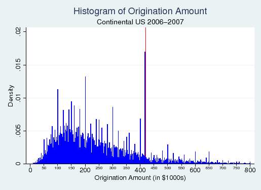
However, a comparison of loans just above and below the conforming loan limit may still be biased due to customer sorting. Indeed, histograms such as Figure 1 suggest that customers bunch just below the conforming loan limit, choosing a larger down payment to avoid getting a jumbo loan. If borrowers that do this are unobservably different from borrowers that don't, estimates of the GSE treatment effect that use this discontinuity will be contaminated by sorting. Indeed, if sorting on unobservables is similar to sorting on observables (Altonji et al., 2005) then the evidence is stark: the average credit score of borrowers in the sample who are just below the conforming cutoff is nearly 45 points higher than it is for those just above the cutoff. It thus appears that more-creditworthy borrowers are better able to take advantage of conforming loans.
To simultaneously address all three sources of bias, this paper uses a slightly different approach. Rather than directly compare loans above and below the conforming loan limit, I instrument for whether a loan is larger or smaller than the limit using a discontinuous function of home appraisal value. As will be explained in detail in Section 3, certain features of the loan origination process ensure that, at particular home appraisal values, the chance that a borrower gets a conforming loan jumps significantly. In particular, above some appraisal values it is impossible to get a conforming loan without putting more than 20% down, inducing a jump in the number of jumbo loans at those values. Evidence suggests that these key appraisal values are not salient to either lenders or borrowers, and there is little evidence of manipulation of appraisals around these values.
This paper thus compares prices and attributes of loans made to borrowers whose homes happen to be appraised just below one of these values, with those of borrowers whose homes happen to be appraised just above. I argue that the resulting differences are most plausibly attributed to the different rates at which these borrowers get conforming rather than jumbo loans. Because GSE purchase eligibility is the essential difference between the conforming and jumbo markets, this quasi-random assignment to the conforming loan market allows for a clean estimate of the equilibrium impact of GSE purchase activities on loan attributes.
Using this method I find only modest impacts of GSE activity. For a sample of loans originated between 2003 and 2007 I estimate that GSE purchase eligibility lowered interest rates in the conforming market by 8 to 12 basis points, which is slightly smaller than previous estimates of the conforming/jumbo spread. I find no significant effect on loan default or foreclosure rates. GSE activity appears to have promoted fixed rate mortgages over adjustable rate mortgages: I estimate an increase of 5.3 percentage points on a base of 61.9 percent fixed-rate loans. GSE intervention also appears to have discouraged low documentation loans and loans bought through a broker. I find no effect on the prevalence of contract features such as pre-payment penalties, negative amortization, interest-only loans, balloon loans, and debt-to-income ratios.
This paper joins a growing literature that attempts to measure the impact of GSE intervention on residential mortgage markets. Previous work has largely focused on determining the effect of GSE intervention on contract interest rates. McKenzie (2002) performs a meta-analysis of eight studies that attempt to quantify the size of the conforming/jumbo rate spread, and concludes that the spread has averaged 19 basis points over the years 1996-2000.5 Studies in this literature generally run regressions in which a "jumbo" dummy is the coefficient of interest, and they control for observables that may covary with jumbo status. Though extremely useful, such studies are potentially vulnerable to selection bias and sorting bias. Later studies, such as Passmore et al. (2005) and Sherlund (2008), yield similar estimates in the 13-24 basis point range while attempting to better address sources of bias.6
Another important strand of the literature has attempted to determine the effect of GSE intervention on the supply of mortgage credit. Ambrose & Thibodeau (2004) uses a structural model to argue that, subsequent to the establishment in 1992 of a set of "Affordable Housing Goals" for the GSEs, the total supply of credit increased slightly more in metropolitan areas with higher proportions of underserved borrowers. Bostic & Gabriel (2006) investigates the same set of housing goals but uses the regulation's definition of what constitutes a "low-income neighborhood" to compare areas that the GSEs were supposed to target with areas where they had no particular mandate, finding no effect of GSE targeting on outcomes such as homeownership rates and vacancy rates.
The present paper contributes to this literature in two ways. First, its estimation strategy is designed to eliminate biases that may have affected previous studies. Second, it expands the set of outcomes examined to include contractual forms and features, as well as measures of loan performance.
Since the original version of the present paper appeared, Adelino et al. (2011) has used a related empirical methodology to study a different question: the effect of GSE loan purchases on house prices. The paper finds that being eligible for a conforming loan increases house prices by slightly over a dollar per square foot.
Section 2 of this paper presents a brief history of the GSEs and provides background on conforming loan limits. Section 3 describes the estimation strategy in greater detail, while Section 4 discusses the dataset and the econometric specifications used. Section 5 presents results, and Section 6 concludes.
2.1 History of the GSEs
The Federal National Mortgage Association (Fannie Mae) was established in 1938 as a federal agency fully controlled by the U.S. government (Fannie Mae, 2010). Its mission was to provide liquidity in the mortgage market by purchasing loans insured by the Federal Housing Administration (FHA). In 1948 that mandate was expanded to include loans insured by the Veterans Administration, and by the early 1950s Fannie Mae had grown to such a point that pressure mounted to take it private. In 1954 a compromise was reached whereby Fannie privatized but was still controlled by the government through Treasury ownership of preferred stock. Fannie was also granted special privileges, such as exemption from local taxes, which it maintains to this day.
The Housing and Urban Development Act of 1968 took the privatization of Fannie Mae a step farther, splitting it by spinning off its functions buying FHA- and VA-insured loans into the wholly government-controlled Ginnie Mae, while preserving the rest of its business in the now supposedly fully-private Fannie Mae.7 However, Fannie Mae continued to enjoy implicit government backing for its debt.
In 1970 the government chartered the Federal Home Loan Mortgage Corporation (Freddie Mac) as a private company. Its mission--buying and securitizing mortgages to promote liquidity and stability--was similar to Fannie Mae's mission, though initially Freddie Mac was only meant to buy mortgages originated by savings and loan associations. With time this distinction eroded. Like Fannie Mae, Freddie Mac was perceived by most as having the implicit backing of the government.
In the wake of the the savings and loan crisis, Congress in 1992 passed the Federal Housing Enterprises Financial Safety and Soundness Act, which established the Office of Federal Housing Enterprise Oversight (OFHEO) as the new regulator for the GSEs. The act also expanded the GSEs' mandate to improve access and affordability for low-income borrowers by creating the Affordable Housing Goals studied in Ambrose & Thibodeau (2004) and Bostic & Gabriel (2006). The rules require the GSEs to buy a certain proportion of their loans from households defined as mid- or low-income, and from neighborhoods defined as low-income.
The GSEs' market share ballooned throughout the 1990s and early 2000s. During this time both institutions expanded their loan purchases and securities issuance, and also began holding more MBS and mortgage loans in portfolio, which they financed by issuing debt.8 Spurred by competition from private-label securitizers, in the mid-2000s the GSEs began expanding their operations into the subprime and Alt-A mortgage markets, which they had traditionally avoided. With the collapse of the housing bubble in mid-2007 the GSEs' subprime MBS holdings put them at risk of insolvency. The Housing and Economic Recovery Act (HERA) of 2008 replaced the regulator OFHEO with FHFA and granted it the power to place the GSEs in conservatorship, which FHFA did in late 2008, finally making explicit the government's long-standing implicit backing of GSE debt. Since then the GSEs have been held in conservatorship, and their future remains uncertain.
2.2 Conforming Loan Limits
By law the GSEs are only allowed to purchase loans smaller than the conforming loan limit (Federal Housing Finance Agency, 2010). Larger loans are referred to as jumbo. The conforming loan limit varies by both year and location. Prior to 2008 the size limit increased at most once a year, and was constant across all locations within the continental United States and Puerto Rico.9
In 2008 the passage of HERA retroactively changed the conforming size limits of loans originated after July 1st, 2007, allowing the GSEs to guarantee more loans. Because the act passed in 2008, it is unlikely that the retroactive changing of the conforming limit in some areas affected loans terms at the time of origination.10 Our only variables measured after origination, default and foreclosure, are likely functions of house price appreciation, loan terms, and borrower credit risk, and as such would not be expected to be directly affected by retroactive eligibility for GSE purchase. After HERA it is no longer the case that all continental U.S. locations are treated equally--the Act designated a set of "high-cost" counties with higher conforming loan limits.
3 Estimation Strategy
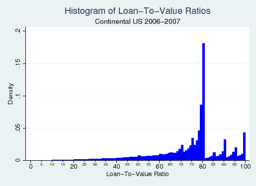
The estimation strategy in this paper employs a discontinuous function of home appraisal value as an instrument for conforming loan status. Appraisal value is related to conforming status for obvious reasons: more expensive houses are more likely to require mortgage loans larger than the conforming limit. However, the relationship between appraisal value and conforming loan status is not smooth. It is discontinuous because loan-to-value (LTV) ratios of exactly 80 (equivalent to a down payment of 20%) are extremely modal in the U.S. mortgage market. An LTV of 80 is common in part because borrowers are typically required to purchase private mortgage insurance (PMI) for loans above 80 LTV. In addition, 80 is considered "normal" and may function as a default choice for many people who would otherwise choose a different down payment. Figure 2 provides a histogram of the loan-to-value ratios of first-lien mortgage loans, illustrating the importance of 80 LTV.
To see why the widespread use of 80 LTV induces a discontinuity in the relationship between appraisal value and conforming status, note that the LTV ratio equals the origination amount divided by the appraisal value. In order to have an LTV of 80 while staying under the conforming limit, a home
cannot be appraised at more than the conforming limit divided by 0.8. For a conforming limit of $417,000, for instance, this appraisal limit, as I will refer to it, would be
![]() . Borrowers with homes appraised above $521,250 must choose whether to put 20% or less down and get a jumbo loan, or put greater that 20% down and get a conforming
loan--conforming loans with 20% down payments are impossible for such borrowers. Because of the stickiness of 80 LTV, borrowers whose homes are appraised above this appraisal limit are discontinuously more likely to get a jumbo loan. Figure 3 illustrates the
first-stage relationship between appraisal value and jumbo status for the 2006-2007 subsample. So long as borrowers do not sort themselves across the appraisal limit, one can use appraisal value as an instrument for whether the borrower gets a conforming or jumbo loan.11
. Borrowers with homes appraised above $521,250 must choose whether to put 20% or less down and get a jumbo loan, or put greater that 20% down and get a conforming
loan--conforming loans with 20% down payments are impossible for such borrowers. Because of the stickiness of 80 LTV, borrowers whose homes are appraised above this appraisal limit are discontinuously more likely to get a jumbo loan. Figure 3 illustrates the
first-stage relationship between appraisal value and jumbo status for the 2006-2007 subsample. So long as borrowers do not sort themselves across the appraisal limit, one can use appraisal value as an instrument for whether the borrower gets a conforming or jumbo loan.11
How easy is it to manipulate appraisal values? Dennis & Pinkowish (2004) provides an overview of the home appraisal process. Independent appraisals are needed because a mortgage lender cannot rely on selling price as a measure of the collateral value of the home. Typically, the lender or mortgage broker contracts a third party to provide an appraisal (Hutto & Lederman, 2003). Borrowers are not allowed to contract appraisers themselves for fear they will shop around for an appraiser willing to inflate the appraisal and thus lower the borrower's LTV. The appraiser estimates the probable market value of the home by taking into account the neighborhood, the condition of the home, improvements to the home, and recent sale prices of comparable homes in the area. Appraisals usually cost $300-500, and the fee is paid by the borrower when the loan application is filed.
The appraisal process is explicitly designed to make it difficult for the borrower to manipulate the appraisal value. However, appraisal manipulation by the lender remains a concern. Anecdotal evidence suggests lenders sometimes leaned on appraisers to inflate values to make loans more attractive for resale on the secondary market.12 Appraisers unwilling to inflate values may have seen a loss of business as a result. Such manipulation may indeed have occurred, but is only relevant for this paper if it occurred across the particular appraisal limit used in the regression discontinuity. If the efforts of lenders to encourage appraisal inflation were less targeted, targeted at another goal, or occurred in small enough numbers, such manipulation would not pose a threat to the empirical strategy. As will be shown in Section 4, there appears to be no bunching around the appraisal limit, suggesting that appraisal values around this limit were not compromised by manipulation by either lenders or borrowers.
Borrowers can manipulate appraisal values in one legal way: by buying a larger or smaller house. However, this form of manipulation is coarse. It would be difficult for a borrower to inch across the threshold by this means; the appraisal value might change by tens of thousands of dollars, or not at all. So long as our estimate is based on the discontinuity in the local area around the cutoff, we can be reasonably sure borrowers are not using home choice to position themselves just below the threshold. Furthermore, the smooth density function we find around the appraisal limit again suggests that this form of manipulation is not a problem.13
Another potential cause of concern about the estimation strategy is the availability of outside financing that is not observable in the dataset. During the 2003-2007 period it became became tolerated practice to fund down payments with a second-lien mortgage. These so-called "silent seconds" were often 15-LTV (or even 20-LTV) second-lien mortgages on an 80-LTV first-lien mortgage. Because the data do not allow for the linkage of first and second lien mortgages made on a given property, it is likely that a significant portion of the 80-LTV loans seen in the data were in fact supplemented by a second-lien mortgage at the time of origination.
However, the invisibility of these second loans does not present a problem for the estimation strategy. Such seconds are the means by which some borrowers managed to stay within the size limit of a conforming loan. So long as not every borrower used second loans to stay within the size limit--perhaps because such seconds were unavailable or were already maxed out, or the borrower was unaware or uninterested in them--then the estimation will provide an unbiased local average treatment effect of GSE purchase activity on those borrowers that would not use seconds in this way if they received an appraisal above the appraisal limit. Such borrowers exist in equal numbers above and below the appraisal limit, but only above the limit are they more likely to actually get jumbo loans.
Though appraisal manipulation and silent seconds are unlikely to present problems for the estimation strategy, at least four limitations of the strategy should be mentioned. First, this method is not appropriate for studying the GSEs' effect on loan terms during the financial crisis itself. From late 2007 onward there was a collapse in the jumbo loan market. Though this itself suggests that the GSEs may have played an important role ensuring access to credit during the crisis, the tiny number of jumbo loans in the 2008-2011 period eliminates the control group necessary for the estimation strategy. In effect, there is no longer a first-stage relationship between appraisal value and jumbo status because there are, to a first approximation, no longer jumbo loans. This paper therefore focuses on the period 2003-2007, and estimates the effects of GSE activity during non-crisis times.
Second, all estimates apply to borrowers taking loans near the conforming loan limit. Despite the fact that the sample period of 2003-2007 saw an unprecedented extension of large mortgage loans to poorer borrowers, it is still the case that most borrowers taking loans close to the conforming limit were relatively affluent. Therefore this estimation strategy is not able to address the question of what effect GSE interventions may have had on the loan terms of less affluent borrowers.
Third, this strategy is ill-suited to estimating the GSEs' effect on access to mortgage credit. The continuity that we see in the loan density function across the appraisal limit suggests that there is little GSE effect on credit availability, at least for more affluent borrowers in the non-crisis 2003-2007 period. However, developing a formal test of this proposition would necessitate adapting a density discontinuity estimation approach such as McCrary (2008) for use in an instrumental variables framework. Such an exercise might be of little use in any event, as GSE credit access effects might be expected most strongly for less affluent borrowers or during crises.
Lastly, these estimates cannot be interpreted as more general estimates of the effects of loan securitization. Though the proportion of conforming loans displays a discontinuity around the appraisal limit, the securitization rate itself does not display a discontinuity (though it does change slope). The results should instead be interpreted as the effects on price, contract structure, and default of being in a segment of the market eligible for purchase by the GSEs.
4.1 Data
The data used in this paper come from Lender Processing Services Applied Analytics, Inc. (LPS).14 These are loan-level data collected through the cooperation of mortgage servicers, including the ten largest servicers in the United States.15 The data cover over half of outstanding mortgages in the United States and contain more than 32 million active loans. Key variables include origination amount, home appraisal amount, loan terms, securitization status, and monthly payment performance.
The analysis sample contains first-lien, non-FHA non-VA insured mortgage loans backed by owner-occupied, single-family homes and originated between the years 2003 to 2007. To be included in the sample, both the origination amount and the appraisal value must be $1,000,000 or less. Table 1 provides summary statistics for this sample of approximately 14.9 million mortgage loans. The numbers for the full sample are broadly consistent with statistics found in studies using other data sources.16 The rightmost columns provide averages for loans that fall within a $5000 band on either side of their appraisal limit. This provides a base rate against which the size of the regression estimates can be judged.17
Figure 1 presents a histogram of loan frequency by origination amount for the continental U.S. in the years 2006 and 2007.18 Visual inspection confirms that there is an atom of borrowers positioned just below the conforming size limit of $417,000. The figure also displays evidence of rounding. Dollar amounts ending in even $5,000, $10,000, and $50,000 increments are more common than other amounts. The presence of rounding makes formal analysis of the discontinuity (as in McCrary (2008)) unreliable. However, because $417,000 falls between tick marks (where we would expect to find a smooth density despite rounding), and because the density there is larger than in any other bin, the atom is very likely not an artifact of rounding. It appears that some borrowers are bunching just below the limit in order to avoid jumbo loans.
Bunching below the limit can only create bias if borrowers below the limit are different from borrowers above the limit. LPS data contain limited information about borrower characteristics, but they do contain one important measure: credit (FICO) score. Taking our 2006-2007 continental U.S. sample, the average FICO score of borrowers in the $5000 bin just below the conforming limit of $417,000 is 740.9, while the average FICO of borrowers in the $5000 bin just above is only 696.5. This swing of nearly 45 FICO points represents a very sizable drop-off in credit quality. Though it is possible to explicitly control for observables such as FICO score, this sorting on observables suggests there may be sorting on unobservables as well. This motivates the use of an instrumental variables specification based on appraisal value.
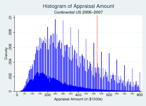
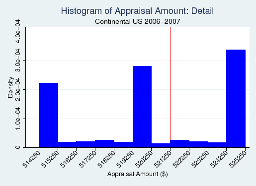
Figure 4 presents a histogram of loan frequency by appraisal value for the same sample. Again there is evidence of rounding, this time making it difficult to visually determine whether there is an atom. Figure 5 provides a close-up of the area around the $521,250 cutoff, which confirms there is no evidence of abnormal bunching. The average FICO score of borrowers in the $5000 bin just below the cutoff is 719.6, while the average FICO score of borrowers in the bin just above is 719.3. It thus appears that appraisal value is not meaningfully compromised by borrower sorting, and is a valid running variable for our regression discontinuity analysis.
4.2 Specification
The instrumental variables regression discontinuity specification used in this paper fits a flexible polynomial on either side of the appraisal cutoff and measures the size of the discontinuity using a dummy variable taking value 1 for observations below the cutoff. The first-stage specification is:
| (1) |
Where ![]() is an indicator for whether the loan origination amount is under the conforming limit,
is an indicator for whether the loan origination amount is under the conforming limit, ![]() and
and ![]() are 7th-order polynomial functions of appraisal amount,
are 7th-order polynomial functions of appraisal amount, ![]() is an indicator for whether the appraisal amount is under the appraisal limit, and
is an indicator for whether the appraisal amount is under the appraisal limit, and
![]() is a vector of control variables including refinance status, dummies for FICO score in 5-point bins, and over 600,000 dummies for every zip code/month of origination
combination in the dataset, allowing us to control for local market conditions extremely flexibly.19 Although the appraisal limit varies by year and
location, all data is pooled by re-centering the data such that, for each year and location, the relevant appraisal limit is equal to zero. This allows the full 2003-2007 sample to be run in a single regression. Table 2 provides a summary of the applicable conforming limits
and appraisal limits for all years and locations in the sample.
is a vector of control variables including refinance status, dummies for FICO score in 5-point bins, and over 600,000 dummies for every zip code/month of origination
combination in the dataset, allowing us to control for local market conditions extremely flexibly.19 Although the appraisal limit varies by year and
location, all data is pooled by re-centering the data such that, for each year and location, the relevant appraisal limit is equal to zero. This allows the full 2003-2007 sample to be run in a single regression. Table 2 provides a summary of the applicable conforming limits
and appraisal limits for all years and locations in the sample.
The second-stage specification is:
| (2) |
Where ![]() is an outcome, such as interest rate, and
is an outcome, such as interest rate, and ![]() is the predicted
value from the first stage. The effect on outcome
is the predicted
value from the first stage. The effect on outcome ![]() of getting a loan in the conforming market as opposed to the jumbo market is estimated by the coefficient
of getting a loan in the conforming market as opposed to the jumbo market is estimated by the coefficient ![]() . The estimate can be thought of as a local average treatment effect of GSE activity on those borrowers who would not respond to a slightly higher appraisal by increasing their down payment above 20% in order to
stay in the conforming market.
. The estimate can be thought of as a local average treatment effect of GSE activity on those borrowers who would not respond to a slightly higher appraisal by increasing their down payment above 20% in order to
stay in the conforming market.
Many of the outcome variables (![]() ) used in this study are binary, suggesting a probit or logit specification. However, the size of the dataset (nearly 15 million observations) coupled
with the number of independent variables (over 600,000) makes such an estimation impractical. For this reason a linear probability model is used instead.
) used in this study are binary, suggesting a probit or logit specification. However, the size of the dataset (nearly 15 million observations) coupled
with the number of independent variables (over 600,000) makes such an estimation impractical. For this reason a linear probability model is used instead.
5 Results
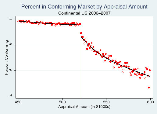
As a first step, Figure 3 confirms that there is power in the first stage by presenting a scatterplot of percent conforming against appraisal value for the continental U.S. in 2006 and 2007. Visual inspection shows a clear discontinuity at the appraisal limit of $521,250. Virtually all borrowers with homes appraised at $521,000 end up with conforming loans, whereas borrowers with homes appraised at $521,500 are discontinuously more likely to get jumbo loans. Table 3 shows the results of a formal first-stage regression using the full sample. There is a discontinuity of 8.8 percentage points, significant at the 1% level, in whether or not the borrower gets a conforming loan.
Tables 4 and 5 present the regression results. Each coefficient in the tables represents a separate instrumental variables regression, each using appraisal value as the running variable and including the complete set of control variables. The estimate in Table 4 of a 10-basis point jumbo/conforming spread is about half the size of many estimates in the literature (McKenzie, 2002). If previous estimates suffered from customer sorting (specifically, more-creditworthy borrowers choosing conforming loans over jumbo loans) this would tend to bias those estimates upwards. However, the disparity could also be due to other factors, such as the difference in sample period.
While conforming status appears to push basic interest rates down, the estimate of its effect on introductory ARM teaser rates is positive 4.6 basis points. Why might teaser rates move in the opposite direction from other rates? One possibility is that lower teaser rates are associated with contracts that are more expensive in other ways. Bubb & Kaufman (2011) shows that in a sample of credit card contracts, for-profit investor-owned credit card issuers were more likely to offer low teaser rates but high interest rates and penalties later on, while cards issued by credit unions have higher teaser rates but lower charges otherwise. Seen in that light, higher teaser rates and lower base rates may be a natural pairing.
Loans eligible for GSE purchase appear to enter default and foreclosure at the same rate as other loans--neither estimate is significant. A negative effect of GSE intervention on default would have been slightly more in line with prior work. Both Elul (2009) and Krainer & Laderman (2009) compare the delinquency outcomes of GSE-securitized loans and privately securitized loans, attempting to control for relevant risk characteristics, and conclude that GSE-securitized loans generally perform better. However these studies look at realized securitization status, not purchase eligibility, and do not attempt to account for sorting bias.
Note that the interest rate effect, in the absence of any significant loan performance effect, suggests that the price difference is not simply due to less risky borrowers receiving a discount. It suggests instead that the price difference is a true effect of GSEs passing on the implicit government subsidy to borrowers.
Table 5 examines the GSE effect on a number of mortgage contract features. There appears to be no effect on the prevalence of a number of "exotic" contract features: pre-payment penalties, interest-only loans, loans allowing negative amortization, and loans with balloon payments all have point estimates indistinguishable from zero. However, there is a GSE effect on at least three aspects of the contract. The conforming market appears to favor fixed-rate mortgages over adjustable-rate mortgages: the prevalence of adjustable-rate mortgages is estimated to drop by 5.3 percentage points. This result is consistent with Green & Wachter (2005), and suggests the GSEs may play a role in allowing borrowers to avoid interest rate risk.
The results further show that GSE activity lowers the prevalence of brokered loans by 4.9 percentage points, and of low documentation loans by 7.8 percentage points. Both low documentation and the use of brokers has been associated with poor loan performance during the crisis. However, it appears that the drops in low documentation and brokerage induced by GSE activity are not enough to have had an affect on default or foreclosure.
6 Conclusion
This paper contributes to the literature on GSE intervention in the mortgage market in two ways. First, it employs a novel econometric strategy designed to produce estimates free of selection bias, sorting bias, and externalities. Second, it expands the set of outcomes examined by including contract features and measures of loan performance. For borrowers with loans near the conforming limit, during the 2003-2007 period, GSE activity lowered interest rates by 8 to 12 basis points, while modestly decreasing the prevalence of adjustable-rate mortgages, low documentation loans, and loans originated through a broker. Effects on contract structure are mixed. There is no measurable effect on loan performance. As the post-conservatorship future of Fannie and Freddie is debated, this set of effects should be weighed against the cost of government support of the GSEs, as well as the potential to achieve such outcomes through other means.
Bibliography
Journal of Political Economy 113(1).
Journal of Real Estate Finance and Economics 23.
Regional Science and Urban Economics 34.
Journal of Urban Economics 59.
Federal Reserve Bank of Boston Public Policy Discussion Paper No. 09-5 .
New York University Law and Economics Working Paper 11-6. .
Studies on Privatizing Fannie Mae and Freddie Mac U.S. Department of Housing and Urban Development.
Thomson South-Western.
Quarterly Journal of Economics 119.
Federal Reserve Bank of Philadelphia Working Paper 09-21 .
http://www.fanniemae.com/.
http://www.fhfa.gov/.
Journal of Economic Perspectives 19(4).
Journal of Real Estate Finance and Economics 2.
Mortgage Bankers Association of America.
Unpublished manuscript.
Federal Reserve Bank of San Francisco Working Paper 09-22 .
Journal of Real Estate Finance and Economics 36(3).
Journal of Economic Perspectives 23(1):27-50.
Journal of Econometrics 142(2):698-714.
Journal of Real Estate Finance and Economics 25.
Journal of Real Estate Finance and Economics 25.
Real Estate Economics 33.
Journal of Real Estate Finance and Economics 25.
Federal Reserve Board Finance and Economics Discussion Series 2008-01 .
Appendix
 |
 |
 |
 |
| Full Sample Mean | Full Sample S.D. | Full Sample Obs. | Near Appraisal Limit Mean | Near Appraisal Limit S.D. | Near Appraisal Limit Obs. | |
| Origination Amount ($) | 212,322 | 129,932 | 14,941,284 | 303,385 | 88,241 | 162,235 |
| Appraisal Value ($) | 308,559 | 191,472 | 14,941,284 | 458,768 | 50,650 | 162,235 |
| Jumbo | .095 | .294 | 14,941,284 | .089 | .285 | 162,235 |
| FICO Score | 711.6 | 61.9 | 12,733,244 | 722.3 | 56.0 | 139,257 |
| Loan-to-Value Ratio | 72.0 | 16.9 | 14,815,612 | 65.9 | 16.9 | 161,282 |
| Interest Rate (%) | 6.25 | 1.38 | 14,284,352 | 6.01 | 1.35 | 153,771 |
| Adjustable Rate Mortgage | .279 | .448 | 14,812,239 | .354 | .478 | 160,722 |
| ARM Teaser Rate (%) | 5.34 | 2.26 | 4,116,418 | 4.88 | 2.15 | 55,110 |
| Pre-Payment Penalty | .133 | .340 | 14,593,905 | .152 | .359 | 159,565 |
| Interest-Only Allowed | .126 | .332 | 14,941,284 | .175 | .380 | 162,235 |
| Negative Amortization Allowed | .050 | .219 | 14,941,284 | .066 | .248 | 162,235 |
| Balloon | .009 | .092 | 14,941,283 | .009 | .096 | 162,235 |
| Brokered | .310 | .462 | 9,866,479 | .327 | .485 | 106,208 |
| Low or No Documentation | .320 | .466 | 8,117,111 | .379 | .485 | 87,858 |
| Debt-to-Income Ratio | 34.9 | 13.4 | 10,033,173 | 35.2 | 12.7 | 112,091 |
| 61+ Day Default | .107 | .309 | 14,941,284 | .098 | .297 | 162,235 |
| Foreclosure | .071 | .258 | 14,941,284 | .065 | .246 | 162,235 |
Notes: Sample of first-lien, non-FHA insured, non-VA insured loans made to borrowers with owner-occupied single-family residences between the years 2003 and 2007. The sample contains only loans with both origination amount and appraisal value $1,000,000 or less. Near Appraisal Limit contains the subset of loans that fall in the $5000 band on either side of their own appraisal limit. Interest Rate defined as contract interest rate for fixed-rate mortgage loans, and as post-teaser margin plus index for adjustable rate mortgage loans. Index value taken at time of origination. 61+ Day Default and Foreclosure equal to 1 if loan ever attains that status within a 36-month window following origination.
| Standard areas Conforming Limit | Standard areas Appraisal Limit | High-cost areas Conforming Limit | High-cost areas Appraisal Limit | |
| 2003 | $322,700 | $403,375 | $484,050 | $605,063 |
| 2004 | $333,700 | $417,125 | $500,550 | $625,688 |
| 2005 | $359,650 | $449,563 | $539,475 | $674,344 |
| 2006 | $417,000 | $521,250 | $625,500 | $781,875 |
| 2007 | $417,000 | $521,250 | $625,500 | $781,875 |
Notes: High-cost areas are defined during the sample period as Alaska, Hawaii, Guam, and the U.S. Virgin Islands. The standard limit applies to the continental U.S. and Puerto Rico. During the sample period the high-cost limit is always 50% larger than the standard limit. Appraisal limit is defined as the applicable conforming limit divided by 0.8.
Notes: First stage regression of conforming status on a dummy indicating whether a loan is above the appraisal limit. Controls include a 7th-order polynomial on either side of the appraisal limit, dummy variables for every combination of zip code and origination month, as well as refinance status and FICO score in 5-point bins. Base Rate is the sample average in the $5000 band below the appraisal limit. Standard errors in parentheses. ***, **, and * denote statistical significance at the 1%, 5%, and 10% levels, respectively.
Notes: Each cell is an instrumental variables regression of the dependent variable on conforming status, instrumenting for conforming status with appraisal value. Controls include a 7th-order polynomial on either side of the appraisal limit, dummy variables for every combination of zip code and origination month, as well as refinance status and FICO score in 5-point bins. Interest Rate defined as contract interest rate for fixed-rate mortgage loans, and as post-teaser margin plus index for adjustable rate mortgage loans. Index value taken at time of origination. 61+ Day Default and Foreclosure equal to 1 if loan ever attains that status within a 36-month window following origination. Base Rate is the sample average in the $5000 band on either side of the appraisal limit. Standard errors in parentheses. ***, **, and * denote statistical significance at the 1%, 5%, and 10% levels, respectively.
| Adjustable Rate | Pre-Payment Penalty | Interest Only | Negative Amortization | Balloon | Brokered | Low Documentation | DTI Ratio | |
| -0.053*** | -0.014 | 0.003 | 0.008 | 0.003 | -0.049*** | -0.078** | 2.633 | |
| s.e. | (0.009) | (0.009) | (0.009) | (0.009) | (0.009) | (0.012) | (0.014) | (1.713) |
| Base Rate | 0.354 | 0.152 | 0.175 | 0.066 | 0.009 | 0.327 | 0.379 | 35.196 |
| 14,812,239 | 14,593,905 | 14,941,284 | 14,941,284 | 14,941,283 | 9,866,479 | 8,117,111 | 10,033,173 |
Notes: Each cell is an instrumental variables regression of the dependent variable on conforming status, instrumenting for conforming status with appraisal value. Controls include a 7th-order polynomial on either side of the appraisal limit, dummy variables for every combination of zip code and origination month, as well as refinance status and FICO score in 5-point bins. Low Documentation includes no documentation loans. Base Rate is the sample average in the $5000 band on either side of the appraisal limit. Standard errors in parentheses. Sample sizes vary due to missing data for some dependent variables. ***, **, and * denote statistical significance at the 1%, 5%, and 10% levels, respectively.