Fiscal Rules, What Does the American Experience Tell Us?
Keywords: Budge rules, fiscal rules, deficits, balanced budget rules
Abstract:
We examine the effect of balanced budget rules on budget outcomes in the U.S. from the mid-1980s through the present. Rules at both the federal level and the state level are considered. Given the relatively short duration of the federal rules and corresponding lack of data points, we adopt a narrative approach. Our examination fails to uncover evidence that the statutory rules at the federal level have influenced the size of deficits. The laboratory of the states provides more fertile ground for econometric testing of the influence of balanced budget rules. We test the hypothesis that the strength of a state's balanced budget rule influences its response to unanticipated budget shocks. We conclude that rules at the state-level have had a significant influence on budget outcomes.
Introduction
Large budget deficits and rising public debt levels have led to renewed interest in budget rules and the means of financing public expenditures. The United States with its federal system offers an interesting environment to study the effects of budget rules. In the U.S. setting there are two very different systems. The federal government has no restrictions from constitutional provisions and few emanating from statutory legislation. By contrast, nearly every state government faces significant constitutional or statutory limitations on their ability to run budget deficits as well as other constitutional or statutory restrictions on budget actions. Our paper endeavors to review and add to the literature on the effectiveness of these rules.
Budget rules can affect budget outcomes in a variety of dimensions. Balanced-budget rules and limits on debt issuance can affect the size of budget surpluses and deficits and the conduct of policy both in a persistent way and over the business cycle. Other budget rules, such as requirements of super majorities for tax provisions, constitutional restrictions on revenues, minimum funding requirements for programs, citizen rights for equal access to education and health, etc., may affect the size and composition of government programs.1 Here we focus on first type of restrictions, those on borrowing and budget deficits.
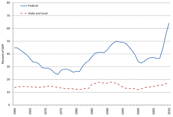
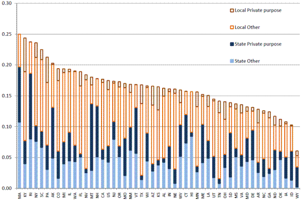
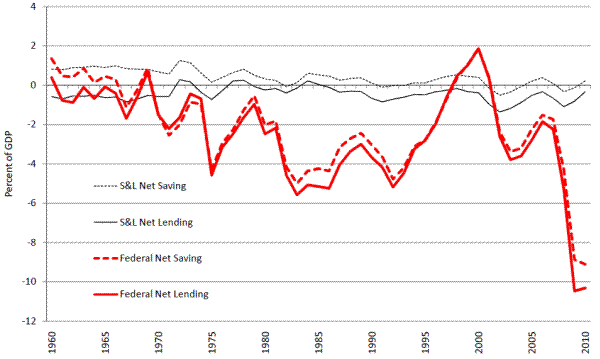
A review of debt and deficit data clearly show that "trend" budget outcomes are different at the federal government and state and local government levels and that conduct over the business cycle is different. Figure 1 displays the evolution of federal and state and local debt over the past 50 years. Two features of the data are readily apparent: Federal debt is much higher and is much more variable than state and local debt. Figure 2 shows debt levels across states.2 The top panel shows that the level of total debt varies significantly across states, but also that there is considerable variability in the composition of debt between state and local and between public debt for private purposes (e.g. industrial development bonds, low income multi-family housing bonds and student loan bonds) and other debt (largely general obligation bonds). Our work will focus on the state budgets and thus state debt. Our results suggest that budget rules are correlated with state debt levels, but that some of the restriction may be offset by behavior at local level.3 Of course, given its higher debt level, the federal government has run much larger deficits, on average, than at the state and local level (Figure 3).
[Figure 1]
[Figure 2]
[Figure 3]
The smaller deficits at the state and local level are likely the outcome of balanced budget rules. These balanced budget rules typically bind on general fund budgets which are similar to operating budgets, thereby excluding capital budgets and other accounts.4 These operating accounts most closely correspond to the current account in the national accounts. In Figure 3 the current account surplus of state and local governments is displayed as net saving, which hovers around zero. Balanced budget rules may affect the conduct of fiscal policy over the business cycle in two dimensions. First, it can make policy pro-cyclical if governments react to falling tax revenues by cutting back on spending or boosting tax rates. Second, these rules will create incentives for governments to seek revenue sources that are less cyclical. Governments can also create a less cyclical policy regime by using rainy day funds. Moreover, states have incentives to create fiscal space to allow counter-cyclical policy. This is true even at the state level, where one might fear that potential leakages would reduce the power of state and local multipliers.5 A recent body of research on state fiscal multipliers by Clemens and Miron (2009), Shoag (2010), and Suarez-Serato and Wingender (2010) suggest that the multiplier on state and local spending may be in the 1-1/2 to 2 range. Nevertheless, Follette and Lutz (2010) demonstrate that at the aggregate level state and local spending has been pro-cyclical while federal government policy has been counter-cyclical. Those results are updated and shown in Table 1. If state fiscal policy can be an effective counter-cyclical policy tool, but state governments behave pro-cyclically, this probably reflects the restrictions that budget rules place on them that they have not been able to relax through the use of rainy day funds. Follette and Lutz (2010) also show that state and local cyclical budgets are less cyclical than those of the federal government, even after controlling for the size of the sector.6 This would be a natural reaction to balanced budget requirements.
[Table 1]
The remainder of this paper will detail the budget rules at first the federal and then the state level and examine how the rules map into budget outcomes. We fail to find evidence that statutory rules at the federal level have had an effect. Their imposition in the 1980s and 1990s were likely reflections of changing policy preferences which may have simultaneously caused changes in budget outcomes. Importantly, the shift to a "pro"-deficit policy after 1998 was not hampered by the rules. By contrast, we find that state budget rules are generally binding. The key difference is probably that state rules are typically constitutionally imposed and thus cannot be adjusted easily by the legislature.
I. Federal Government Budgeting
A. Background
Rules covering federal budgets have evolved significantly over time. Importantly the constitution provides little restriction on the size or structure of government or limits on borrowing.7 The current budget process was established by the Budget Control and Impoundment Act of 1974. The annual budget process begins in February with the release of the Administration's five-year budget plan. Each house of Congress has a budget committee whose responsibility is to craft a budget resolution in the spring that provides the framework for the overall budget by: outlining the path for policy for the next five years and setting targets for the two types of implementing legislation - appropriations bills and reconciliation bills. The two budget resolutions are melded into one which then controls debate of the implementing legislation. The twelve appropriations bills cover the annual spending needs of the agencies for discretionary programs and must be within the limits set by the joint budget resolution.8 The reconciliation bills cover spending and tax legislation used to implement the portion of the budget resolution that is not covered by the annual appropriations bills-taxes and most transfers and subsidies (called mandatory spending).9 Other tax and spending bills may also be considered on an ad hoc basis during the year, but if they are inconsistent with the budget resolution then they are subject to parliamentary rules which create additional hurdles, particularly in the Senate.
B. Gramm-Rudman-Hollings: 1985-1990
The 1974 Budget Act had been enacted owing to a growing unease about budget deficits, as well as owing to conflicts between the executive and legislative branches. In 1985, the budget process was changed radically in an attempt to rein in persistently large deficits that the Budget Act had failed to stem. The Balanced Budget and Emergency Deficit Control Act of 1985, commonly known as Gramm-Rudman-Hollings (GRH), made two changes to the budget process. First, it instituted annual deficit targets that could only be exceeded by a small margin. Second, it created a sequestration mechanism to meet the targets. The Administration would estimate the deficit in mid-October for the fiscal year that had just begun based on enacted legislation and economic and technical assumptions made earlier in the year.10 If the projected deficit exceeded the target by more than $10 billion (about 0.2 percent of GDP), then expected outlays of discretionary programs-half from defense and half from nondefense-would be cut so as to meet the target.11 Notably, compared to many state budget rules, only the projected deficit needed to meet the target. Among the nondefense expenditures, the cuts would be uniform across all programs.
Federal Unified Budget Deficit Targets and Results Under GRH (Billions of dollars, fiscal years)
| 1986 | 1987 | 1988 | 1989 | 1990 | 1991 | 1992 | 1993 | |
| GRH target,1985 | 172 | 144 | 108 | 72 | 36 | 0 | ||
| GRH target, 1987 | 144 | 136 | 100 | 64 | 28 | 0 | ||
| Actual deficit | 221 | 150 | 155 | 153 | 221 | 269 | 290 | 255 |
| Memo: Deficit, % of GDP | 5.0 | 3.2 | 3.1 | 2.8 | 3.9 | 4.5 | 4.6 | 3.9 |
Did GRH work? Clearly, the Gramm-Rudman-Hollings approach did not achieve its stated goal of balancing the budget. Indeed, lack of progress during the first two years led the government to enact revised targets in 1987 in the Balanced Budget and Emergency Deficit Control Reaffirmation Act when the target for fiscal 1988 appeared to be unreachable. In 1989, the automatic sequester was triggered for the first time. (GRH applied to the ex-ante budget, hence the deviation between the GRH target deficit and actual deficit in the table above reflects overly optimistic budget assumptions.) Then in 1990, the initial Congressional Budget Office (CBO) projections showed the deficits for 1990 and 1991 coming in well above the GRH targets. But, while the Administration's fiscal 1991 budget showed the fiscal 1990 deficit coming in significantly above the target, its proposed fiscal 1991 deficit was just under the limit, largely owing to overly optimistic economic and technical assumptions. By June, the fiscal situation had deteriorated enough so that the overly optimistic scenario had to be abandoned and President Bush choose to go back on his "Read my lips, no new taxes" pledge.12 At that point the GRH framework was abandoned in favor of an alternative framework (see below).
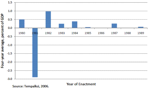
While the GRH rules did not lead to a balanced budget, did these rules restrain policy more than would have been the case without the targets? This we may be able to answer by looking at tax policy, changes to entitlement programs, and discretionary spending. While the sequestration process was directed at discretionary spending, the targets were expected to be met through fiscal consolidation using all budget levers. With respect to taxes, after GRH was passed several small tax bills were enacted, but they were smaller than the ones earlier in the decade (excluding the 1981 Reagan Tax cuts). Thus, these tax policy changes appear, at best, to be a continuation of prior policy of addressing outsized deficits partially through taxes (Figure 4a).
[Figure 4a and 4b]
During the 1980s there were some major changes to reduce entitlement spending, including changes to Social Security, Medicare, unemployment benefits, and grants to state and local governments.13 Some of these cuts were enacted during the GRH period-in particular a reduction in mandatory grants to S&L for general revenue sharing and small cuts to Medicare-but these appear to be a continuation of the prior policy and were no more stringent than those enacted immediately prior to GRH.14
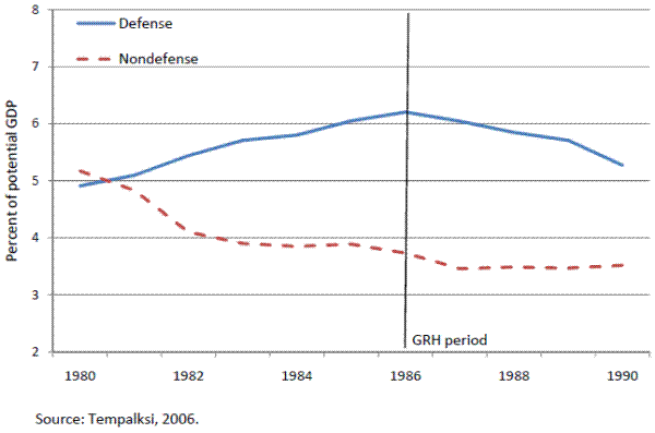
Discretionary spending during the second half of the 1980s slowed relative to the first half of the decade. During the first half of the decade discretionary spending was relatively constant as a share of potential GDP as increases in defense were offset by declines in nondefense (Figure 4b).15 During the second half of the decade (after GRH was put in place) discretionary spending fell by 1 percent of potential GDP, mostly in the defense category. While the decline in defense may reflect the additional pressures from GRH, arguably it may reflect the changing circumstances in foreign affairs. Turning to non-defense, this category of spending fell sharply in 1986 and 1987 and then rose at the pace of potential GDP during the following three years, when the screws from GRH should have been tightening. The initial decline probably owes to the cuts implemented when GRH was instituted and in the following year, but this time pattern gives little support that GRH induced additional cuts over time.
In sum, our reading of the record is that there is little clear evidence that GRH resulted in additional budget consolidation efforts. The first time the GRH targets bound significantly in 1988, the targets were revised. When they again bound in 1990, they were abandoned. There is no clear evidence that policy actions were more restrictive than they had been prior to GRH. Perhaps, the failure to hit the targets in 1990 led to the 1990 budget summit (see below), and those budget cutting actions could be credited to the GRH targets. Alternatively, a change in policy preferences concerning deficits may have led to both the enactment of GRH and the 1990 summit.
Analysis by others is mixed. Reischauer (1990) and Gramlich (1990) find little support for the effectiveness of GRH, while Hahm (1992) and Auerbach (2008) are more supportive. Regression analysis by Hahm and Auerbach show more fiscal consolidation during the GRH period than prior.16 But, those results may reflect the changing desires of Congress rather than the change in the rules. Importantly, as stated above, when the targets became binding, Congress relaxed the targets.
C. The Budget Enforcement Act (BEA): PAYGO and Discretionary Caps
Following the recognition that GRH had failed, a new budget regime, the Budget Enforcement Act (BEA), was put in place in 1990 as a part of the Omnibus Budget and Reconciliation Act (OBRA 1990). Under the new structure budget decisions, rather than budget forecasts or budget outcomes, were constrained. OBRA 1990 put in place policies that were expected (but not required) to achieve budget balance by 1995 through a set of tax increases and mandatory spending cuts that were implemented as part of the legislation, as well as restrictions on discretionary spending that would have to be implemented through annual appropriations bills over the following five years. Annual limits for discretionary spending were put in place for the 1991 to 1995 period.17 A PAYGO rule was established so that the set of tax and mandatory spending laws enacted in a session would not increase the deficit. Enforcement had several components. First, bills that violated the spending caps and PAYGO rules were subject to parliamentary hurdles. Second, excesses in budget authority or projected outlays for discretionary spending would trigger across-the-board sequesters of discretionary spending, similar to the GRH rule. Third, if the changes to taxes and mandatory spending resulted in an increase in the deficit, thereby violating PAYGO, a sequester of mandatory spending was triggered. These restrictions had a relief valve in that spending for "emergency" purposes would be exempt.
The BEA rules proved more durable than the explicit deficit targets used by GRH and were in place when the budget moved from deficit to surplus. But, it is still difficult to discern how much of an independent factor they played, versus being a reflection of the policy environment. After they were put in place 1990, the deficit widened owing to the recession, Gulf War, and the savings and loan bailout (Table 2, lines 3 and 6 show the deterioration). Interestingly, while temporary expansion of unemployment benefits were enacted and not offset (using the emergency designation available to avoid PAYGO), there were no other countercyclical policies (unlike a typical recession, see Follette and Lutz (2010)). Outside of the Gulf War the discretionary caps were maintained. Thus, a case can be made that they worked initially by preventing the typical counter-cyclical policy reaction. However, immediately following enactment and over the following two years, economic and "technical" developments greatly worsened the budget outlook, so that by 1993 the budget was in worse shape than it had been before OBRA 1990 and no policies were enacted to offset these poor outcomes (see lines lines 5 and 6 of table 2).18 The failure of BEA to require a response to deficits arising from incorrect technical and economic assumptions (as opposed to policy decisions) rendered it ineffective as an anti-deficit device in this period. It is possible that having met the BEA requirements, Congress did not feel the need to react further. It is therefore possible that the BEA actually worsened the deficit position by "turning off" this natural reaction function. In any case, it clearly did not restrain the deficit during the early years.
[Table 2]
Following the 1992 elections, President Clinton put forth a new budget plan that called for balancing the budget in five years, with tax increases and mandatory spending cuts-particularly to Medicare, and continued adherence to slightly revised and extended discretionary caps (Omnibus Budget and Reconciliation Act of 1993, table 2, middle panel, line 9). At the time, the 1990 rules were seen as effective, but insufficient, because deficits had not fallen, rather they had remained near 4 percent of GDP (line 8). The Clinton plan was not projected to bring balance, but to cut the deficit as a share of GDP in half, to a level where it would lead to a small decline in the debt-to-GDP ratio. Importantly, this budget plan was not required by the 1990 rules and thus cannot be credited to the success of BEA. As with the 1990 caps and PAYGO, these restrictions held through the President's term. No other material policy actions were taken during the remaining years of the first term. That said, the 1995-96 government shutdown (instigated when the new Republican majority tried to cut discretionary spending significantly) and the 1996 welfare reform reduced the deficit a smidgeon. These actions were not required by OBRA 1993 and provide some confirmation of the view that the government-Congress and the administration-was looking for ways to cut the deficit beyond what was required by OBRA. Thus the OBRA rules were not binding during this period.
At the beginning of Clinton's second term the Tax Reduction and Balanced Budget Act was passed in the summer of 1997. The Act extended the discretionary caps through 2002, provided small tax cuts, and made important reductions to Medicare and other entitlements (line 16 of lower panel of table 2). The Act was projected to balance the budget by 2002 if the discretionary caps held. However, many analysts thought this unlikely because they viewed the caps as too onerous. That spring (line 17) and over the following four years (line 20), though, economic and technical factors pushed the budget far into surplus.
The 1998-2002 period is the key period for judging the efficacy of the BEA framework in our opinion. The 1990, 1993 and 1997 policy actions were not necessitated by the BEA and consequently the budget restraint provided by them was not likely due to the caps. Over the 1998-2002 period, budget surpluses became the norm. Initially, it appears that the BEA framework worked to encourage saving the surpluses. Some argue that the surpluses were the result of the surprising pickup in productivity and economic growth over the second half of the 1990s. But budget policy was clearly the reason for the surpluses, because the extra revenues could have been spent with tax cuts and spending increases, like they were in the 1960s and they would be in the 2000s. The question is whether the tight fiscal policy was a result of the rules or of the decisions of the Clinton Administration and Congress. While it is possible that the budget rules were responsible, it is at least equally plausible that the split in control between a Democratic president and a Republican Congress caused a stalemate on what to do with the surpluses. The BEA edifice began to crumble as the discretionary spending caps were breeched in 1999 and 2000 using emergency designations by the first Congress that was working with a cap that it had not enacted. Previously, the caps had been usually set by the same Congress-the exception being the 1995-96 Congress. When President Bush was inaugurated in 2001, control of both branches of government shifted to the Republicans and the budget stalemate ended, and neither the President nor Congress had been a party to enacting the controlling budget framework. The existing budget framework was quickly discarded and an exceptionally large tax cut enacted despite the PAYGO rules. The tax cut was then accompanied by increases in discretionary and mandatory spending. Moreover, there were no efforts to offset the rapid deterioration in the budget.
For us, the 1998-2002 period shows that when the BEA framework of discretionary spending caps and PAYGO restrictions were inconsistent with desired policy, the budget rules were ignored or changed. By contrast, Auerbach (2008) claims some modest success for the BEA framework. This differing conclusion is due to his excluding the years 1998-2002 as being part of BEA while crediting the BEA process for deficit reducing actions in 1993 and 1997.19 Although it is certainly possible that the BEA contributed to the 1993 and 1997 reductions, the framework did not bind in these years and the rules would have had to influence policy in an indirect manner. Recently, PAYGO was reinstated in 2010 and has met the same fate. Although the health reform met the criteria, the tax cuts enacted in the fall did not, despite the shift in budget climate to austerity. Thus, statutory PAYGO has not been able to prevent a majority from enacting significant deficit increasing legislation.
II. State Balanced Budget Rules
A. Background
All U.S. states except Vermont have a legal balanced budget requirement.20 These requirements are sometimes contained in the state constitution, while in other cases they are statutory (i.e. they have been enacted into law by the state's legislature). In some instances, they are based on court rulings pertaining to constitutional-based debt limits.21
Although there is considerable variation in how the balanced budget rules are implemented across the states, there are three general types. The first requires that the governor's proposed budget be balanced; the second requires that the budget passed by the legislature be balanced; and the third requires that that the budget be balanced at the end of the fiscal year, often referred to as a no-carryover provision.22 Regardless of the type, the rules refer only to operating budgets and explicitly exclude capital budgets.
There are several ways in which states can address a deficit to satisfy its balanced budget requirement. In all states the legislature may reduce expenditures (although the legislature will not always be in session when the deficit, or projected deficit, arises). In many states the Governor or an appointed board may reduce outlays if a budget shortfall has emerged. In almost all cases, state legislatures may increase revenues. They can also draw down general fund and rainy day fund balances accrued in previous fiscal years. Some states may engage in short-term borrowing to cover a budget gap, although this must generally be paid back in the following fiscal year. It is quite rare for states to explicitly engage in long-term borrowing to cover an operating deficit, although it does occasionally occur: California borrowed $11 billion in 2004 to address a shortfall in its operating budget.23 It remains an open question, though, if states engage in long-term borrowing ostensibly for capital expenditures and then use accounting tricks to move the funds into the operating budget. (For example, a state could borrow to finance highway construction and then divert motor fuel tax revenues (that were intended to finance capital spending) from its highway trust fund to the general fund. Many states require a referendum for new long-term debt issuance which may inhibit this type of behavior. Finally, there are a host of short-term maneuvers which may be used to satisfy balanced budget requirements in letter, but not spirit. For instance, states may defer spending scheduled for the end of the fiscal year to the start of the following fiscal year, defer payments owed to vendors, to employees, and to local governments, take a "holiday" from making pension fund contributions, or change the timing of tax payments.
The literature to date has generally concluded that the stringency of balanced budget requirements has a significant effect on state fiscal behavior, with the no-carryover provision being particularly important. Bohn and Inman (1996) conclude that the no-carryover rule is associated with larger state general fund balances. These larger balances accrue due to relatively lower spending, not higher taxes. Similarly, Poterba (1994) finds that more stringent rules, primarily the no-carryover provision, are associated with more rapid adjustment to budget deficits. The margin of adjustment to these shocks is found to be spending, not taxes. Clemens and Miran (2010) and Clemens (2009) extend Poterba's results to a more recent period. (Poterba used data from 1988-1992 and they extend the sample to 2004). These authors confirm Poterba's basic result and also conclude that state spending has a large fiscal multiplier of around 1.7 (Clemens and Miran, 2010) and that public sector union strength predicts which areas of the budget are cut (Clemens 2009).
B. Balanced Budget Rules and the Level of Fiscal Outcomes
We now turn to examining the relationship between balanced budget rule stringency and various fiscal outcomes. In this section we examine the relationship between balanced budget rules and the level of various fiscal outcomes, namely year-end balances, deficits and debt levels. In the next section we examine how balanced budget rules influence the reaction to shocks to fiscal conditions. Although the level relationship is likely more important, the evidence we produce is mostly suggestive in nature. In contrast, while the fiscal shock question is narrower in scope, we are able to provide more formal evidence. In both cases, our goal is to establish whether rule stringency is associated with differences in state fiscal behavior.
We quantify budget rule stringency using the index developed in ACIR (1987). The index runs from 0 to 10, with 10 denoting the most stringent balanced budget rules and 0 denoting no rules. The presence of a no-carryover provision is the most important predictor of receiving a high index value.24 We follow Clemens (2009) and categorize states with an index of 7 or higher as strong budget rule states and the remainder as weak budget rule states.
State governments typically spend and tax out of many accounts. However, only the general fund - a state's largest account and the one used to fund most broad-based services - is directly constrained by balanced budget rules (Bohn and Inman 1996). We therefore focus our attention on general fund expenditures, revenues and year-end balances as measured annually in the National Association of State Budget Officer's (NASBO) Fiscal Survey of the States.
Finally, we also examine total debt levels. As noted earlier, while debt is largely taken on for capital expenditures, and also applies to accounts other than the general fund, resources may be fungible across accounts (e.g. the general fund, capital, and pension accounts) and uses (e.g. capital outlays and operating outlays). Additionally, one of the ultimate aims of balanced budget rules is to prevent the accumulation of debt and debt is therefore an important outcome measure in assessing the efficacy of the rules.
Year-end Balances and Deficits
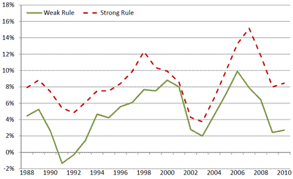
Total year-end balances, the sum of the year-end balance in a state's general fund and rainy day fund, provide a signal of a state's fiscal position. Large year-end balances indicate the state has adequate resources to buffer negative shocks, while low balances may force difficult choices over taxes and spending in the event of an adverse shock. Although balances in excess of 5 percent have traditionally been considered adequate, this judgment likely needs to be revised. Record high balances at the end of fiscal 2006 proved woefully insufficient to buffer the subsequent economic downturn.25
Panel A of Figure 5 displays average total year-end balances as a percent of general fund expenditures. Balances are quite cyclical, rising during good economic times and falling as the economy turns downward. At all times, though, strong rule states maintain larger balances than weak rule states. Thus, strong budget rules states persistently maintain a stronger fiscal position than weak rule states.
[Figure 5a and 5b]
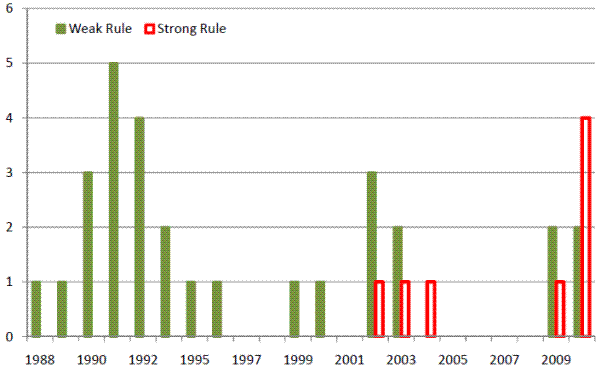
Panel B examines deficits - years in which the sum of balances in the general fund and rainy day accounts are negative.26 Deficits are somewhat cyclical, as they are most prevalent in the years immediately following recessions. Over most of the period, weak rule states were substantially more likely to run deficits. Interestingly, though, during the period of severe fiscal stress in 2009 and 2010, strong rules states were slightly more likely to end the year in deficit than weak rule states.
Debt
Simple correlations of the ACIR rating and debt levels suggest that tighter budget restrictions are associated with lower debt levels for the state general obligation bonds (-.357) or total state debt (-.374). The correlations for broader aggregates, such as for total state and local government bonds (which include debt by governments not subject to the rules measured by the ACIR ratings), are somewhat weaker. This suggests that these covenants may be binding and that states do not fully circumvent the covenants by shifting borrowing to the local level. There may be some shifting, as there is a negative correlation between state and local debt levels. The positive correlation between local debt and ACIR rating (which only applies to state debt) suggests that the negative relation between state debt and ACIR rating is not solely reflective of a taste for debt whereby areas with a higher tolerance for debt would have looser restrictions and higher debt at both levels of government. If that were the case then it is likely that the local debt levels would also be negatively correlated with the ACIR rating. Finally, the bottom rows of the table indicate that states with tighter restrictions experienced less debt growth over the 2000s, a period of strain for state budgets because of the two recessions.
Correlation of Debt with Budget Restrictions
| Type of debt | State and local | State | Local | Memo: Correlation of state debt with local debt |
| Level of Debt in 2008: Total debt | -.311 | -.374 | .062 | -.480 |
| Level of Debt in 2008: GO debt | -.223 | -.357 | -.005 | -.140 |
| Change in Debt, 2000-2008: Total debt | .033 | -.077 | .122 | .339 |
| Change in Debt, 2000-2008: GO debt | .055 | -.226 | .217 | .086 |
Debt is the ratio of debt to state GDP. Budget restrictions are measure by ACIR rating where a higher number is more restrictive.
Source. Census of Governments. GO debt is total debt less public debt for private purposes.
C. Budget Rules and Fiscal Shocks
In this section we examine how balanced budget rules influence the response of state governments to adverse fiscal shocks. In particular, we focus on the extent to which states adjust to shocks by making changes to taxes and spending, versus drawing down reserve funds and engaging in various accounting maneuvers.
Measuring Fiscal Shocks
Like Clemens and Miran (2010) and Clemens (2009), we utilize the budget shock framework pioneered by Poterba (1994). The budget shock framework utilizes general fund data collected by NASBO on both realized expenditures and revenues and the projections of expenditures and revenues upon which the budget for the fiscal year was based. In a state which requires that the passed budget be balanced, projected expenditures may not exceed projected revenues (including any year-end balances from the previous fiscal which are to be used in the current fiscal year). The NASBO data also contains information on expenditure and revenue changes enacted after the budget was passed, referred to as mid-year changes, such as spending reductions made to address a deficit. The data is currently available from the 1988 to 2010 fiscal year.
The revenue shock experienced by a state in a given year is the difference between actual revenues and the amount of revenues forecasted at the time the budget was passed, net of any mid-year policy changes:
| (1) |
where
Similarly, the expenditure shock is defined as:
| (2) |
where
![]() is the mid-year policy change in expenditures (i.e. changes in spending enacted into law after the budget was passed). Positive expenditure shocks occur for a number of
different reasons, including when an economic downturn increases demand for transfer programs such as Medicaid.
is the mid-year policy change in expenditures (i.e. changes in spending enacted into law after the budget was passed). Positive expenditure shocks occur for a number of
different reasons, including when an economic downturn increases demand for transfer programs such as Medicaid.
The deficit shock experienced by a state in a given year is the difference between its expenditure shock and its revenue shock:
| (3) |
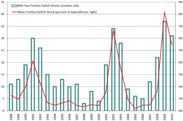
The analysis focuses on positive deficit shocks which tend to arise during periods of fiscal stress. (For completeness, we display the results for negative shocks on the tables, but do not discuss them.) Figure 6 displays the average positive deficit shock (the average deficit shock conditional on the shock being positive) in all years of our sample. The shocks are highly cyclical, consistent with the notion that they are driven by unexpected fluctuations in economic activity. The magnitude of these shocks, and the number of states experiencing them, are only a bit larger following the recent 2007-2009 recession than during much milder 2001 downturn, in part because of relief provided by federal grants.
[Figure 6]
Outcomes
States have three primary methods for balancing their budget in the face of an adverse deficit shock: mid-year spending cuts,
![]() , mid-year tax changes,
, mid-year tax changes,
![]() , and mid-year drawdown of reserve funds,
, and mid-year drawdown of reserve funds,
![]() . As already discussed,
. As already discussed,
![]() and
and
![]() are changes made to spending and taxes after the budget has been passed, but before the end of the fiscal year.27 These outcomes are considered in Poterba (1994).
are changes made to spending and taxes after the budget has been passed, but before the end of the fiscal year.27 These outcomes are considered in Poterba (1994).
One of the contributions of this paper is to examine a third outcome, the drawdown of reserve funds, as this is one of the chief mechanisms by which states respond to shocks.
![]() quantifies the unanticipated change in a state's reserve funds. It is defined as:
quantifies the unanticipated change in a state's reserve funds. It is defined as:
| (4) |
where
Empirical Model
We estimate the influence of deficits on spending and taxes with the following specification:
| (5) |
| (6) |
| (7) |
The hypothesis that states must annually balance their budgets yields the prediction that
In order to assess how the stringency of balanced budget rules affects the spending response to a deficit we estimate the following (and an analogous equation is used for the other outcomes):
| (8) |
where
Sample
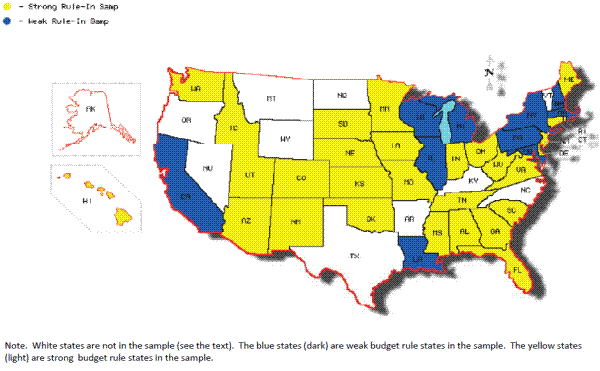
We restrict our sample to those states with either an annual budgeting cycle or an annual legislative cycle. States in which the legislative and budgeting cycles are both biennial are excluded as their response to fiscal shocks is likely to play out over a two-year period instead of the one-year framework assumed by the budget shock methodology. Following Clemens (2009), Alaska, Wyoming and Vermont are also excluded from the sample. Vermont is excluded because it has no balanced budget rules. Alaska and Wyoming are excluded because they exhibit very atypical fiscal flows, largely as a result of heavy reliance on the taxation of natural resource extraction (primarily oil). The estimation sample includes 39 states. Figure 7 displays these states and identifies the stringency of their budget rules. Finally, the NASBO data is available from 1988 through 2010. The estimation sample is limited to years of relative fiscal stress: 1988-1994, 2001-2004, and 1998-2010, although results are general similar if all years 1988-2010 are included.
Table 3 presents summary statistics for the sample. The mean positive fiscal shock is a bit over $45 per-capita (expressed in 2004 dollars). Importantly, the magnitude and variance of positive deficit shocks (defshock ![]() 0) is nearly equal between weak and strong budget rule states (columns 2 and 3). The budget shock framework relies on the assumption that deficit shocks are true forecasting errors. Alternatively, the shocks could contain systematic bias. For instance, forecasts
may be influenced by political pressure-e.g. intentionally optimistic forecasts intended to facilitate spending increases. This scenario becomes particularly problematic if the extent of bias is associated with the stringency of the rules-e.g. states with strong budget rules tend to produce less
optimistic forecasts because the costs of overly optimistic forecast errors are increased by the stringency of the rules. In this case, divergence in fiscal behavior between weak and strong rule states might reflect endogenous forecast bias, not the efficacy of the rules. It is therefore
encouraging that deficit shocks appear similar in both weak and string rule states. Although negative deficit shocks appear to be somewhat larger in weak rule states, the analysis does not focus on these shocks.
0) is nearly equal between weak and strong budget rule states (columns 2 and 3). The budget shock framework relies on the assumption that deficit shocks are true forecasting errors. Alternatively, the shocks could contain systematic bias. For instance, forecasts
may be influenced by political pressure-e.g. intentionally optimistic forecasts intended to facilitate spending increases. This scenario becomes particularly problematic if the extent of bias is associated with the stringency of the rules-e.g. states with strong budget rules tend to produce less
optimistic forecasts because the costs of overly optimistic forecast errors are increased by the stringency of the rules. In this case, divergence in fiscal behavior between weak and strong rule states might reflect endogenous forecast bias, not the efficacy of the rules. It is therefore
encouraging that deficit shocks appear similar in both weak and string rule states. Although negative deficit shocks appear to be somewhat larger in weak rule states, the analysis does not focus on these shocks.
[Figure 7]
[Table 3]
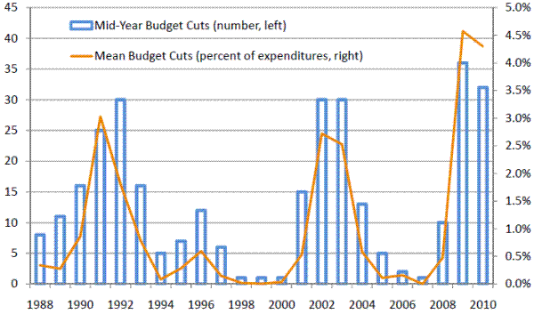
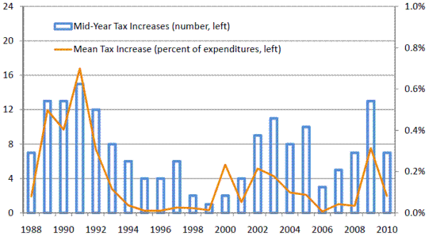
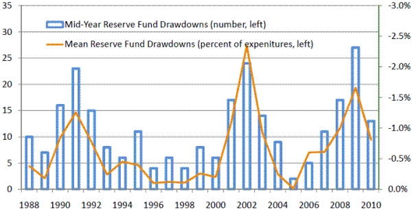
The remainder of the table displays the means for the three outcome variables. These mid-year budget adjustments are all quite cyclical, as can be seen in the three panels of Figure 8.
![]() (Panel A) only reflects spending cuts (see footnote 26). In order to make the panels comparable,
(Panel A) only reflects spending cuts (see footnote 26). In order to make the panels comparable,
![]() (Panel B) and
(Panel B) and
![]() (Panel C) are plotted conditional on being positive and negative, respectively. Thus, the panels display the evolution over time of mid-year spending cuts, tax
increases and reserve drawdowns.
(Panel C) are plotted conditional on being positive and negative, respectively. Thus, the panels display the evolution over time of mid-year spending cuts, tax
increases and reserve drawdowns.
[Figure 8]
Results
Table 4 displays the results of estimating the budget shock equations. Each dollar of positive deficit shock causes state policy makers to reduce spending by around 50 cents (column 1), with the estimate falling to about 40 cents with the inclusion of year and state fixed-effect terms (column 2). Tax policy plays only a minor role in addressing mid-year deficits, as each dollar of shock induces only 5 cents of tax increases within the fiscal year (columns 3 and 4). Note, though, that tax changes often take time to implement and such frictions may limit the utility of this policy lever for addressing with-in fiscal year budget shortfalls.31 Reserve funds are used to plug roughly 20 cents of each dollar of deficit shock and thus occupy a middle ground between spending and taxes (columns 5 and 6).32 In total, the three outcomes are used to clear from around 75 cents to 65 cents of each dollar of shock (columns 7 and 8). The residual 25 cents to 35 cents is dealt with through deficit financing or accounting techniques such as transfers from other governmental accounts.
[Table 4]
Panel A of Table 5 considers the possibility that the response to deficits may have differed during the 2008-2010 period (as compared to the other periods of fiscal stress in the sample, 1988-1994 and 2001-2004). Examining this period is another contribution of our analysis. Not only were the magnitude of deficits larger in this period (Figure 6), but states also received a large infusion of temporary grants from the federal government beginning in fiscal 2009.33 The infusion of aid, which is reflected in the NASBO data, significantly reduced the magnitude of the mid-year deficit shocks (at least in 2009). However, states were aware that the downturn was likely to be unusually protracted and that the fiscal assistance was temporary. As a result, they may have been reluctant to use all of the fiscal stimulus grants to plug current year budget shortfalls, but instead may have decided to use these funds over several years. Using the funds over a period of several years would require a more intense response to the mid-year deficits of 2008-2010 than occurred in response to the deficits of earlier periods.
Panel A fails to support the hypothesis of a more intense fiscal response in the 2008-2010 period. Although spending and reserves appear to experience a larger adjustment (columns 1 and 5), these results are not robust to the inclusion of year and state fixed-effects (columns 2 and 6). The overall adjustment per dollar of deficit shock achieved through the three fiscal margins appears to have been the same in 2008-2010 as in earlier periods (columns 7 and 8). That said, because the shocks ware larger the adjustments were greater.
[Table 5]
The ultimate aim of the analysis, assessing the efficacy of balanced budget rules, is addressed in Panel B. The response to deficits is permitted to differ by strong and weak budget rule states (equation 7). The estimates suggest that strong rule states reduce spending mid-year by about 50 cents for every dollar of shock, while weak rule states cut spending by only 30 cents (column 1). However, the result is only weakly precise when the year and state terms are included (column 2). In contrast, the budget rule effect on budget recessions is remarkably robust in Clemens (2009). Turning to taxes, the results are somewhat puzzling as weak rule states increase taxes more in response to deficit shocks than do strong rule states. However, the primary conclusion from Table 4 remains: in both weak and strong rule states only a small fraction of a deficit shock is addressed though mid-year tax increases. Finally, there is no evidence that budget rules influence reserve fund drawdowns (columns 5 and 6).
Table 6 explores the possibility that the efficacy of balanced budget rules changed in the 2008-2010 period. The estimating equation interacts the deficit shock measure with both
![]() and
and
![]() , where
, where
![]() is an indicator for fiscal years 2008-2010. A triple interaction of the deficit shock and
is an indicator for fiscal years 2008-2010. A triple interaction of the deficit shock and
![]() and
and
![]() is also included. To ease the interpretation, the marginal effects of a positive deficit shock for differing groups of states, as well as the results of hypothesis testing
based on these marginal effects, are presented in the bottom portion of the table.
is also included. To ease the interpretation, the marginal effects of a positive deficit shock for differing groups of states, as well as the results of hypothesis testing
based on these marginal effects, are presented in the bottom portion of the table.
[Table 6]
In contrast with the results on Panel B of Table 5, there is strong evidence of budget rule efficacy on the spending margin (columns 1 and 2; hypothesis test ii). Strong rule states engage in 41 cents of mid-year spending cuts when a budget shortfall opens (marginal effect a), whereas weak rule states make only 18 cents of cuts (marginal effect c). These results are nearly identical to those in Clemens (2009) (unsurprisingly given that these marginal effects are identified from the exact same set of years as used in Clemens). There is some indication, though, that the difference between weak and strong rule states has been reduced in the current period. While there is a fairly large difference in the magnitude of the current period spending response, 39 cents for weak rule states (marginal effect d) versus 55 cents for strong rule states (marginal effect b), the difference is not precise (hypothesis test iv). Furthermore, the estimates suggest that the behavior of weak rule states on the spending margin has changed in the current period relative to the earlier period. Previously these states reduced spending by 18 cents (marginal effect c), but in the current period they cut spending by 39 cents (marginal effect d); the difference is statistically meaningful (hypothesis test iii). Although strong rule states also appear to have increased the intensity of their response (marginal effects a and b), the difference is not precise (hypothesis test i).
The evidence is thus somewhat mixed as to how much the spending response to deficit shocks differs in the current period and the role of budget rules in this difference. Taking a step back, one possibility is that the lack of statistical precision for some of the hypothesis tests may disappear when more data is available from the current crisis. Overall, the point estimates suggest that both weak and strong budget rule states increased the magnitude of their spending response.
On the tax margin there appears to be insufficient power to draw many precise conclusions (columns 3 and 4). However, there is evidence that the more aggressive weak rule state response on the tax margin, as compared to strong rule states, seen on Table 5 is produced by behavior in the current period (hypothesis test iv). Again, though, the overall size of the tax response is small.
It appears that states have been relatively hesitant to drawdown reserve funds in the current period relatively to their prior behavior (columns 5 and 6; hypothesis test i). States reduced their reserves by around 35 cents in prior episodes (marginal effect a), but reduced reserves by only about 10 cents in 2008-2010 (marginal effect b). There is no evidence that budget rules influence the magnitude of this response in any period.
III. Conclusion
Reviewing the American experience we find little evidence that statutory budget rules affect budget decisions. At times the rules are correlated with better budget outcomes, but this may reflect changes in the preferences of policymakers inducing a simultaneous change in both budget rules and budget outcomes. By contrast, at the state level budget rules appear to have teeth. This leads to lower levels of debt, smaller deficits, and more pro-cyclical budget outcomes at the state level than at the federal level. We see this behavior in the aggregate time series data as well as in the cross-section data.
References
Advisory Commission on Intergovernmental Relations (1987). "Fiscal Discipline in the Federal System: National Reform and the Experience of the States," 1987.
Auerbach, Alan (1994). "The U.S. Fiscal Problem: Where We Are, How We Got Here, and Where We're Going," NBER Macroeconomics Annual, MIT Press, Cambridge.
Auerbach, Alan (2008). "Federal Budget Rules: The U.S. Experience," Swedish Economic Policy Review, Vol. 15.
Bohn, Henning, and Robert Inman (1996). "Balanced-budget Rules and Public Deficits: Evidence from the U.S. States," Carnegie-Rochester Conference Series on Public Policy.
Congressional Budget Office, The Budget and Economic Outlook, various years.
Clemens, Jeffrey and Stephen Miran (2010). "The Effects of State Budget Cuts on Employment and Income," mimeo.
Clemens, Jeffrey (2009). "State Fiscal Adjustment During Times of Stress: Composition and Its Possible Causes," mimeo.
Congressional Quarterly (1977). Congress and the Nation, Volume IV, 1973-1976, CQ Press,Washington DC.
Congressional Quarterly (1989). Congress and the Nation, Volume VII, 1985-1988, CQ Press,Washington DC.
Follette, Glenn and Byron Lutz (2010). "Fiscal Policy in the United States: Automatic Stabilizers, Discretionary Fiscal Policy Actions, and the Economy," Banca d'Italia Public Finance Workshop.
Gramlich, Edward (1990). "U.S. Federal Budget Deficits and Gramm-Rudman-Hollings" American Economic Review Papers and Proceedings, May.
Hahm, Sung Deuk, Mark S. Kamlet, David C. Mowery, Tsai-Tsu Su(1992). "The Influence of the Gramm-Rudman-Hollings Act on Federal Budgetary Outcomes, 1986-1989," Journal of Policy Analysis and Management, Vol. 11, No. 2.
Hou Yilin and Daniel Smith, "Do state balanced budget requirements matter? Testing two explanatory frameworks," Public Choice, 2010.
Hou, Yilin & Daniel Smith, "A framework for understanding state balanced budget requirement systems; re-examining distinctive features and an operational definition." Public Budgeting & Finance, 26(3), 2006.
National Association of State Budget Officers (2010-1988). Fiscal Survey of the States. Washington DC.
National Conference of State Legislatures, "State Balanced Budget Requirements", April 12, 1999. (http://www.ncsl.org/default.aspx?tabid=12660)
Poterba, James, "State Responses to Fiscal Crises: The Effects of Budgetary Institutions and Politics," Journal of Political Economy, vol. 102, no. 4, 1994.
Reischauer, Robert (1990). "Taxes and Spending Under Gramm-Rudman-Hollings," National Tax Journal, Vol. 43, No. 3, September.
Shoag, Daniel (2010). "The Impact of Government Spending Shocks:Evidence on the Multiplier from State Pension Plan Returns."
Suarez Serrato, Juan Carlos, and Phillippe Wingender (2010). Estimating Local Fiscal Multipliers.
Table 1: Fiscal Impetus Around Business Cycles (Percent of GDP)
| Peak year | 1969 (1) | 1973 (2) | 1980 (3) | 1990 (4) | 2000 (5) | 2007 (6) | Average (7) |
| Federal Government Year before peak | 0.02 | 0.55 | 0.19 | -0.23 | 0.30 | 0.31 | 0.19 |
| Federal Government Peak | -0.77 | -0.16 | -0.04 | -0.27 | 0.07 | 0.23 | -0.16 |
| Federal Government 1 year after | -0.01 | 0.00 | -0.31 | -0.47 | 0.48 | 1.07 | 0.13 |
| Federal Government 2 years after | -0.20 | 0.58 | 0.76 | -0.31 | 0.95 | 1.20 | 0.50 |
| Federal Government 3 years after | 0.55 | 0.36 | 0.95 | -0.56 | 0.90 | 0.63 | 0.47 |
| Federal Government Before | -0.38 | 0.20 | 0.07 | -0.25 | 0.19 | 0.27 | 0.02 |
| Federal Government After | 0.11 | 0.31 | 0.47 | -0.44 | 0.78 | 0.97 | 0.37 |
| State and Local Government Year before peak | 0.89 | -0.04 | 0.31 | 0.47 | 0.53 | 0.06 | 0.37 |
| State and Local Government Peak | 0.50 | -0.04 | 0.17 | 0.52 | 0.38 | 0.27 | 0.30 |
| State and Local Government 1 year after | 0.21 | 0.55 | -0.21 | 0.24 | 0.55 | 0.04 | 0.23 |
| State and Local Government 2 years after | 0.34 | 0.48 | 0.16 | 0.17 | 0.35 | -0.61 | 0.15 |
| State and Local Government 3 years after | -0.04 | -0.05 | 0.22 | 0.34 | -0.19 | -0.47 | -0.03 |
| State and Local Government Before | 0.69 | -0.04 | 0.24 | 0.50 | 0.46 | 0.16 | 0.33 |
| State and Local Government After | 0.17 | 0.33 | 0.06 | 0.25 | 0.24 | -0.35 | 0.12 |
| General Government Before | 0.31 | 0.16 | 0.31 | 0.25 | 0.65 | 0.43 | 0.35 |
| General Government After | 0.29 | 0.64 | 0.52 | -0.19 | 1.01 | 0.62 | 0.48 |
Table 2a: Evolution of the Deficit 1990-93 (Percent of GDP fiscal years unified budget basis)
| 1990 | 1991 | 1992 | 1993 | 1994 | 1995 | |
| 1 July 1990 | 3.4 | 3.9 | 3.8 | 3.0 | 2.1 | 1.9 |
| 2 OBRA 1990 | 0.0 | -0.6 | -1.1 | -1.4 | -1.9 | -2.2 |
| 3 Other | 0.4 | 1.7 | 1.8 | 1.7 | 2.1 | 1.1 |
| 4 January 1991 | 3.8 | 5.0 | 4.5 | 3.3 | 2.3 | 0.8 |
| 5 Policy | 0.0 | 0.1 | 0.4 | 0.1 | 0.1 | 0.1 |
| 6 Other | 0.0 | -0.5 | -0.3 | 1.3 | 1.8 | 3.0 |
| 7 January 1993 | 3.9 | 4.6 | 4.6 | 4.7 | 4.2 | 3.9 |
Table2b: Evolution of the Deficit 1993-98 (Percent of GDP fiscal years unified budget basis)
| 1993 | 1994 | 1995 | 1996 | 1997 | 1998 | |
| 8 January 1993 | 4.7 | 4.2 | 3.9 | 3.7 | 3.9 | 4.1 |
| 9 OBRA 1993 | 0.0 | -0.5 | -0.7 | -1.1 | -1.4 | -1.7 |
| 10 Other | -0.7 | -0.1 | -0.4 | -0.2 | -0.0 | -0.2 |
| 11 August 1993 | 4.0 | 3.6 | 2.7 | 2.5 | 2.4 | 2.3 |
| 12 Policy | 0.0 | 0.1 | 0.1 | -0.1 | -0.1 | 0.0 |
| 13 Other | -0.2 | -0.8 | -0.5 | -1.0 | -0.9 | -0.9 |
| 14 January 1997 | 3.9 | 2.9 | 2.2 | 1.4 | 1.4 | 1.4 |
Table 2c: Evolution of the Deficit 1993-98 (Percent of GDP fiscal years unified budget basis)
| 1997 | 1998 | 1999 | 2000 | 2001 | 2002 | 2003 | |
| 15 January 1997 | 1.4 | 1.4 | 1.6 | 1.8 | 1.6 | 1.8 | 1.8 |
| 16 Balanced Budget and Tax Relief Act | 0.0 | 0.2 | -0.0 | -0.2 | -0.2 | -0.9 | -0.7 |
| 17 Other | -1.0 | -1.0 | -1.0 | -1.1 | -1.1 | -1.2 | -1.5 |
| 18 September 1997 | 0.4 | 0.7 | 0.6 | 0.5 | 0.4 | -0.3 | -0.3 |
| 19 Policy | 0.0 | 0.0 | 0.2 | 0.6 | 1.0 | 1.5 | 1.6 |
| 20 Other | -0.1 | -1.5 | -2.2 | -3.5 | -4.1 | -4.2 | -4.5 |
| 21 January 2001 | 0.3 | -0.8 | -1.4 | -2.4 | -2.7 | -3.0 | -3.3 |
| 22 Policy | 0.8 | 1.4 | 3.3 | ||||
| 23 Other | 0.7 | 3.0 | 3.4 | ||||
| 24 January 2004 | 0.3 | -0.8 | -1.4 | -2.4 | -1.2 | 1.5 | 3.4 |
Table 3: Summary Statistics for NASBO State Government General Fund Data
| Mean All States (1) | Mean Weak Budget Rule States (2) | Mean Strong Budget Rule States (3) | P-Value for Test of Equality of Weak Rule and Strong Rule Means (4) | |
|---|---|---|---|---|
| Defshock > 0 - Point Estimate | 47.42 | 45.92 | 51.38 | 0.53 |
| Defshock > 0 - Standard Error | (90.08) | (87.05) | (97.86) | |
| Defshock < 0 - Point Estimate | -18.42 | -20.53 | -12.85 | 0.06 |
| Defshock < 0 - Standard Error | (41.98) | (45.80) | (29.00) | |
| ΔSpend - Point Estimate | -26.96 | -28.93 | -21.78 | 0.17 |
| ΔSpend - Standard Error | (53.83) | (57.23) | (43.43) | |
| ΔTax - Point Estimate | 2.35 | 1.49 | 4.51 | 0.01 |
| ΔTax - Standard Error | (12.57) | (8.74) | (19.00) | |
| ΔReserves - Point Estimate | 8.66 | 13.33 | -3.22 | 0.01 |
| ΔReserves - Standard Error | (66.03) | (57.41) | (83.12) | |
| Number of Observations | 539 | 391 | 148 |
Table 4: State Reaction to Fiscal Shocks
| ΔSpend (1) | ΔSpend (2) | ΔTax (3) | ΔTax (4) | ΔReserves (5) | ΔReserves (6) | ΔSpend - ΔTax + ΔReserves (7) | ΔSpend - ΔTax + ΔReserves (8) | |
|---|---|---|---|---|---|---|---|---|
| Defshock > 0 - Point Estimate | -0.47 | -0.38 | 0.05 | 0.05 | -0.21 | -0.21 | -0.73 | -0.64 |
| Defshock > 0 - Standard Error | (0.04)*** | (0.05)*** | (0.02)** | (0.02)** | (0.07)*** | (0.07)*** | ||
| Defshock < 0 - Point Estimate | 0.01 | -0.06 | 0.02 | 0.03 | -0.78 | -0.73 | -0.79 | -0.82 |
| Defshock < 0 - Standard Error | (-0.02) | (-0.04) | (-0.02) | (-0.02) | (0.10)*** | (0.16)*** | ||
| Number of observations | 539 | 539 | 539 | 539 | 536 | 536 | N/A | N/A |
| Year Fixed-Effects | X | X | X | X | ||||
| State Fixed-Effects | X | X | X | X |
Table 5: Balanced Budget Rules and State Reaction to Fiscal Shocks
| ΔSpend (1) | ΔSpend (2) | ΔTax (3) | ΔTax (4) | ΔReserves (5) | ΔReserves (6) | ΔSpend - ΔTax + ΔReserves (7) | ΔSpend - ΔTax + ΔReserves (8) | |
|---|---|---|---|---|---|---|---|---|
| A. Parameters Permited to Differ in 2008-2010 Fiscal Downturn Defshock > 0 - Point Estimate | -0.32 | -0.30 | 0.06 | 0.06 | -0.35 | -0.31 | -0.73 | -0.67 |
| A. Parameters Permited to Differ in 2008-2010 Fiscal Downturn Defshock > 0 - Standard Error | (0.05)*** | (0.05)*** | (0.02)*** | (0.02)** | (0.07)*** | (0.08)*** | ||
| A. Parameters Permited to Differ in 2008-2010 Fiscal Downturn Defshock < 0 - Point Estimate | -0.04 | -0.08 | 0.02 | 0.04 | -0.67 | -0.61 | -0.73 | -0.73 |
| A. Parameters Permited to Differ in 2008-2010 Fiscal Downturn Defshock < 0 - Standard Error | (-0.02) | (0.02)*** | (-0.02) | (0.02)* | (0.13)*** | (0.20)*** | ||
| A. Parameters Permited to Differ in 2008-2010 Fiscal Downturn Defshock > 0 * Current Downturn - Point Estimate | -0.18 | -0.11 | -0.02 | -0.01 | 0.16 | 0.15 | 0.00 | 0.05 |
| A. Parameters Permited to Differ in 2008-2010 Fiscal Downturn Defshock > 0 * Current Downturn - Standard Error | (0.06)*** | (-0.07) | (-0.02) | (-0.04) | (0.07)** | (-0.14) | ||
| A. Parameters Permited to Differ in 2008-2010 Fiscal Downturn Defshock < 0 * Current Downturn - Point Estimate | 0.09 | 0.02 | -0.02 | -0.03 | -0.27 | -0.33 | -0.16 | -0.28 |
| A. Parameters Permited to Differ in 2008-2010 Fiscal Downturn Defshock < 0 * Current Downturn -Standard Error | (-0.05) | (-0.07) | (-0.02) | (-0.02) | (-0.17) | (0.19)* | ||
| B. Parameters Permited to Differ by Strength of Budget Rules Defshock > 0 - Point Estimate | -0.53 | -0.43 | 0.02 | 0.03 | -0.15 | -0.17 | -0.70 | -0.63 |
| B. Parameters Permited to Differ by Strength of Budget Rules Defshock > 0 - Standard Error | (0.05)*** | (0.05)*** | (-0.02) | (-0.02) | (0.03)*** | (0.05)*** | ||
| B. Parameters Permited to Differ by Strength of Budget Rules Defshock < 0 - Point Estimate | 0.02 | -0.06 | 0.01 | 0.03 | -0.75 | -0.67 | -0.74 | -0.76 |
| B. Parameters Permited to Differ by Strength of Budget Rules Defshock < 0 - Standard Error | (-0.02) | (-0.04) | (-0.01) | (0.02)** | (0.10)*** | (0.14)*** | ||
| B. Parameters Permited to Differ by Strength of Budget Rules Defshock > 0 * Weak Rules - Point Estimate | 0.19 | 0.15 | 0.07 | 0.08 | -0.18 | -0.11 | -0.06 | -0.04 |
| B. Parameters Permited to Differ by Strength of Budget Rules Defshock > 0 * Weak Rules - Standard Error | (0.07)** | (0.09)* | (0.03)** | (0.04)** | (-0.16) | (-0.18) | ||
| B. Parameters Permited to Differ by Strength of Budget Rules Defshock < 0 * Weak Rules - Point Estimate | -0.02 | 0.01 | 0.05 | 0.00 | -0.26 | -0.53 | -0.33 | -0.52 |
| B. Parameters Permited to Differ by Strength of Budget Rules Defshock < 0 * Weak Rules - Standard Error | (-0.03) | (-0.08) | (-0.04) | (-0.06) | (-0.20) | (-0.37) | ||
| Number of observations | 539 | 539 | 539 | 539 | 536 | 536 | N/A | N/A |
| Year Fixed-Effects | X | X | X | X | ||||
| State Fixed-Effects | X | X | X | X |
Table 6: Balanced Budget Rules and State Reaction to Fiscal Shocks
| ΔSpend (1) | ΔSpend (2) | ΔTax (3) | ΔTax (4) | ΔReserves (5) | ΔReserves (6) | |
|---|---|---|---|---|---|---|
| Defshock > 0 - Point Estimate | -0.41 | -0.39 | 0.05 | 0.05 | -0.32 | -0.33 |
| Defshock > 0 - Standard Error | (0.04)*** | (0.05)*** | (0.03)* | (0.03) | (0.07)*** | (0.10)*** |
| Defshock > 0 * Current Downturn - Point Estimate | -0.14 | -0.07 | -0.03 | -0.03 | 0.20 | 0.23 |
| Defshock > 0 * Current Downturn - Standard Error | (0.07)* | (0.09) | (0.02)* | (0.02) | (0.06)*** | (0.11)** |
| Defshock > 0 * Weak Rules - Point Estimate | 0.23 | 0.24 | 0.03 | 0.04 | -0.07 | 0.09 |
| Defshock > 0 * Weak Rules - Standard Error | (0.04)*** | (0.06)*** | (0.03) | (0.04) | (0.13) | (0.11) |
| Defshock > 0 * Weak Rules * Current Downturn - Point Estimate | -0.07 | -0.10 | 0.06 | 0.05 | -0.14 | -0.25 |
| Defshock > 0 * Weak Rules * Current Downturn - Standard Error | (0.10) | (0.10) | (0.05) | (0.05) | (0.21) | (0.21) |
| Marginal Effects (a) Positive Shock | -0.41 | -0.39 | 0.05 | 0.05 | -0.32 | -0.33 |
| Marginal Effects (b) Positive Shock during Current Crisis | -0.55 | -0.46 | 0.02 | 0.02 | -0.12 | -0.11 |
| Marginal Effects (c) Positive Shock with Weak Rules | -0.18 | -0.15 | 0.08 | 0.09 | -0.38 | -0.24 |
| Marginal Effects (d) Positive Shock during Current Crisis with Weak Rules | -0.39 | -0.32 | 0.10 | 0.11 | -0.32 | -0.26 |
| Hypothesis Testing (P-values) (i) Current Crisis Differs from Prior Episodes H0: (a) - (b) = 0 | 0.07 | 0.43 | 0.09 | 0.18 | 0.00 | 0.05 |
| Hypothesis Testing (P-values) (ii) Weak Rules Differs From Strong Rules H0: (a) - (c) = 0 | 0.00 | 0.00 | 0.40 | 0.31 | 0.62 | 0.38 |
| Hypothesis Testing (P-values) (iii) Weak Rules in Current Crisis Differ from Weak Rules in Prior Episodes H0: (d) - (c) = 0 | 0.00 | 0.03 | 0.55 | 0.71 | 0.76 | 0.94 |
| Hypothesis Testing (P-values) (iv) Weak Rules in Current Crisis Differ from Strong Rules in Current Crisis H0: (d) - (b) = 0 | 0.09 | 0.18 | 0.03 | 0.03 | 0.33 | 0.47 |
| Number of observations | 539 | 539 | 539 | 539 | 536 | 536 |
| Year and State Fixed-Effects | X | X | X |
