Skip to: [Printable Version (PDF)] [Bibliography] [Footnotes]

Finance and Economics Discussion Series: 2012-45 Screen Reader version ^♣

Signal Extraction for Nonstationary Multivariate Time Series with Illustrations for Trend Inflation

Tucker McElroy and Thomas Trimbur

U.S. Census Bureau and Federal Reserve Board

June 2012

Keywords: Co-integration, common trends, filters, multivariate models, stochastic trends, unobserved components.

Abstract:

This paper advances the theory and methodology of signal extraction by introducing asymptotic and finite sample formulas for optimal estimators of signals in nonstationary multivariate time series. Previous literature has considered only univariate or stationary models. However, in current practice and research, econometricians, macroeconomists, and policy-makers often combine related series - that may have stochastic trends - to attain more informed assessments of basic signals like underlying inflation and business cycle components. Here, we use a very general model structure, of widespread relevance for time series econometrics, including flexible kinds of nonstationarity and correlation patterns and specific relationships like cointegration and other common factor forms. First, we develop and prove the generalization of the well-known Wiener-Kolmogorov formula that maps signal-noise dynamics into optimal estimators for bi-infinite series. Second, this paper gives the first explicit treatment of finite-length multivariate time series, providing a new method for computing signal vectors at any time point, unrelated to Kalman filter techniques; this opens the door to systematic study of near end-point estimators/filters, by revealing how they jointly depend on a function of signal location and parameters. As an illustration we present econometric measures of the trend in total inflation that make optimal use of the signal content in core inflation.

JEL Classification: C32

Disclaimer

This report is released to inform interested parties of research and to encourage discussion. The views expressed on statistical issues are those of the author and not necessarily those of the U.S. Census Bureau or the Federal Reserve Board.

1 Introduction

In many scientific fields, research and analysis make widespread use of a signal extraction paradigm. Often, interest centers on underlying dynamics (such as trend, non-seasonal, and cyclical parts or, more generally, systematic movements) of time series also subject to other, less regular components such as temporary fluctuations. In such cases, the resulting strategy involves the estimation of signals in the presence of noise. For instance, economists and policy-makers routinely want to assess major price trends, cycles in industrial and commercial activity, and other pivotal indicators of economic performance. Typically, the measurement of such signals combines judgmental elements with precise mathematical approaches.

Here, we concentrate on the latter aspect, with the goal of developing the formal apparatus for detecting signals in a comprehensive econometric framework, motivated by two basic considerations. First, the signal extraction problems relevant to experience usually involve more than one variable; at central banks, for instance, staff use a range of available series to monitor prevailing inflationary conditions. Second, economic data often involve nonstationary movements, with (possibly close) statistical relationships among the stochastic trends for a set of indicators.

In this paper we generalize the existing theory and methodology of signal extraction to multivariate nonstationary time series. In particular, we set out analytical descriptions of optimal estimator structures that emerge from a wide range of signal and noise dynamics, both for asymptotic and for finite sample cases. Our results give a firm theoretical basis for the expansion of the Wiener-Kolmogorov (WK) formula to the nonstationary multivariate framework and provide a simple and direct method (distinct from the state space approach) for calculating signal estimates and related quantities, and for studying endpoint effects explicitly. In presenting these formulas, we also treat the case of co-integrated systems, which, as with other econometric problems, has special implications for the characteristics of the signal estimators. Previously, many applications of signal extraction have been undertaken without such a rigorous foundation. Such a basis unveils properties of signal estimators, and hence allows for a host of developments, such as the design of new architectures from the collective dynamics for signal and noise vector processes and the analysis of signal location effects in finite series.

The previous literature in this area, which handles only single series or stationary vector series, has a long history. For a doubly infinite data process, Wiener (1949) and Whittle (1963) made substantial early contributions; the corresponding WK formula, which gives the asymptotic form (for historical, or two-sided smoothing) of the relationship between optimal signal estimation and the component properties, has become a theoretical benchmark in time series econometrics. The original WK filters assumed stationary signal and noise vector processes, whose properties entered directly into the expressions through their autocovariance generating functions (ACGF). With awareness about the importance of nonstationarity in time series analysis growing through the early 1980s, Bell (1984) proved the optimality of an analogous bi-infinite filter for nonstationary data. However, despite the widespread knowledge of correlated movements among related variables in macroeconomics and in other disciplines, which has motivated an enormous amount of research on multivariate time series models over the last several decades, the relevant theory has not yet been provided for multiple nonstationary series.

Past theoretical work on signal extraction for finite samples has concentrated on single series (see Bell (2004) and McElroy (2008) and the references therein). Most economic applications have relied on standard Kalman filtering and smoothing algorithms, for instance the trend-cycle analyses in Harvey and Trimbur (2003), Azevedo et al. (2006), and Basistha and Startz (2008). The implied weights on the input series may be computed in each case with an augmentation of the basic algorithms, as in Koopman and Harvey (2003); yet this method omits closed-form expressions or explicit information about the functional form of the filters. Bell (1984) introduced some exact results; subsequently, the compact formulas in McElroy (2008) provided a considerable simplification, amenable to simple implementation (and possibly other uses, such as analytical investigation of end-point effects). However, to our knowledge, the finite sample theory has not yet been presented for multivariate signal-noise processes, whether stationary or nonstationary.

As a primary goal, this paper presents new results on signal estimation in doubly-infinite time series for multivariate nonstationary models. These expressions capture the basic action - independent of signal location and sample size - of the estimators, leading to compact expressions in the time and frequency domains that give complete descriptions of the operators' effects. Our generalization of the WK formula provides a firm mathematical foundation for the construction of jointly optimal estimators for multiple series, and reveals explicitly how signal extraction architectures, having the form of matrix filter expressions, emerge from the collective dynamics of signal and noise vectors.

We also introduce signal extraction results for finite samples, generalizing the analysis in McElroy (2008) to multivariate systems including nonstationary¹ series. The formulas give a very general mapping from stochastic signal-noise models to optimal estimators at each point in finite sample vector series. This reveals the explicit weighting patterns on the observation vectors for estimation close to the end of the series, which is a crucial problem for generating signals central to current analysis and economic decision-making. Having such an optimal accounting for the finite series length seems especially helpful for multiple series; compared to the univariate setup, in addition to the position effect, we now have collections, or matrices, of time-dependent and asymmetric filters with complex inter-relationships for each time period. More generally, our results incorporate the complete functional dependence of the filter set on parameters, sample size, and estimate location, so they include the interaction of signal-noise dynamics with distance to end-point and series length in the formation of the optimal weight vectors. In contrast to the state space approach, our matrix expressions enable straightforward and direct computation of multivariate signals, as well as providing additional information, such as the estimation error covariance across individual signals and across different times. The matrix expressions are also more widely applicable than the state space smoother, because some processes of interest (e.g., long-range dependent processes) cannot be embedded in a state space framework.

Signals of interest typically have an interpretation; for instance, stochastic trends capture permanent or long-run movements and underpin the nonstationarity found in most economic time series. The trend components usually dominate the historical evolution of series and prove crucial for understanding and explaining the major or lasting transitions over an existing sample. Toward the end-points, they may account for an important part of recent movements, that are likely to propagate into the new observations that will become available for the present and future periods. Hence, accurate estimation of stochastic trends often represents a signal extraction problem of direct interest, giving a pivotal input for assessing patterns in past behavior and for current analysis and near-term projection.

We apply our theoretical developments on two stochastic trend models widely used in the literature. Simple dynamic representations are used to demonstrate the combination of nonstationary and stationary parts, that occurs in many economic time series. For richer models, in separating trend from noise, the key aspects illustrated by our examples continue to drive the best signal estimators: the form of nonstationary component, its strength relative to the noise for each series, and the interactions among series for each component. Of course, the treatment of stochastic trends, where present, also crucially affects other areas such as measurement of cyclical or seasonal parts, given the reciprocity of the estimation problem for the various components in a set of series.

We also address the case of common (or co-integrated) trends, and explore its implications for signal estimation. Starting with early work such as Engle and Granger (1987), Stock and Watson (1988), and Johansen (1988), the importance of such co-movements for econometric methodology has been long established, based on their impact on statistical theory and estimator properties, along with the evidence for their frequent occurrence found by researchers. While related to VAR-based formulations, such as Engle and Granger (1987) and Johansen (1988), the common trends form, as presented in Stock and Watson (1988), allows us to directly handle tightly linked long-term signals, and is also useful beyond this context. For instance, this formulation makes available a different class of tests for the integration order of processes, as in Nyblom and Harvey (2000). Here, we allow for the presence of co-integration in the formulation of our general theorems.

We present an application of the above models to the measurement of trend inflation with data on both core and total inflation. Using these time series models as the basis of the signal estimation ensures consistency with the dynamic properties and cross-relationships of the bivariate inflation. Our extensions to signal extraction theory allow us to derive the precise estimators of the trend in total inflation. These results (which differ from trend measurement with a simple reliance on core alone) quantify the degree of emphasis on core and the corresponding down-weighting of total, expressed in either the time or frequency domains.

The rest of the paper is arranged as follows. Section 2 develops the generalized WK formula for a set of nonstationary time series, expressing the optimal multivariate filters in both the frequency and time domains. Exact signal extraction results for a finite-length dataset are derived in Section 3. Then Section 4 reviews some major models for multivariate stochastic trends, and the methodology is illustrated by the statistical measurement of trend inflation using both core and total inflation data. Section 5 provides our conclusions, and mathematical proofs are in the Appendix.

2 Multivariate signal extraction from a bi-infinite sample

This section gives a highly general solution to the signal extraction problem for multiple nonstationary series and generalizes the WK formula to this case. The aim of signal extraction is to elicit components of interest - the signals - from series that also contain other components. Signal-noise decompositions have the form of unobserved component (UC) processes, where the signal processes (which may take the form of a combination of two or more distinct latent processes) typically have an interpretation, such as a stochastic trend, that suggest some dynamic formulation. The noise combines all the remaining components in the series; then, to achieve the goal of extracting the target signals, we may use an appropriate filter to remove the unwanted effects of the noise. The WK formula produces the optimal estimator of the signals in terms of the dynamics of the UC processes, so it shows how component structure maps into filter design. In this way, the filters that emerge from the formula have the major advantages of coherency with each other and - by setting parameters in accordance with a fitted model - of consistency with the set of input series.

In formulating the theory behind multivariate signal extraction, we first treat the benchmark case of a hypothetical doubly infinite process. In the next section we examine the estimation problem based upon a finite sample. The bi-infinite case is useful for studying the fundamental and long-term impact of filters, as it abstracts from near-end-of-sample effects and allows one to derive mathematical expressions in terms of the specifications of components and parameter values that capture the essence of the signal extraction mechanism. This theoretical framework generally proves most useful for analysis in the frequency domain, for which signal estimators typically give rise to gain functions of a compact form, making possible the transparent and straightforward comparison of optimal filters across different models. The doubly infinite assumption represents a natural limiting case, with estimators based on the maximum information set, and in practice, for long enough samples, it applies approximately to most of the time points in a wide neighborhood around the mid-point.

We first set out our notation and some basic concepts; also see Brockwell and Davis (1991). Consider a vector-valued, possibly nonstationary, time series denoted $\{\mathbf{y}_{t}\}= \{ \mathbf{y}_{t}, -\infty < t < \infty \}$ , with each $\mathbf{y}_{t}$ of dimension A multivariate filter for a set of series has the expression

$\displaystyle \boldsymbol{W}(L)=\overset{\infty }{\underset{h=-\infty }{\sum }}\boldsymbol{% W}_{h}L^{h},$

(1)

where

is the standard lag operator, and $\boldsymbol{W}_{h}$ is the $% N\times N$ matrix of coefficients for lag

. The cross-elements $% \boldsymbol{W}_{h}^{jk}$ and $\boldsymbol{W}_{h}^{kj}$ are generally unequal. The filter produces output $\mathbf{z}_{t}$ as follows:

$\displaystyle \mathbf{z}_{t}=\boldsymbol{W}(L)\mathbf{y}_{t}=\overset{\infty }{\underset{% h=-\infty }{\sum }}\boldsymbol{W}_{h}L^{h}\mathbf{y}_{t}=\overset{\infty }{% \underset{h=-\infty }{\sum }}\boldsymbol{W}_{h}\mathbf{y}_{t-h}.$

(2)

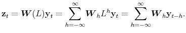
Therefore, the weight matrix $\boldsymbol{W}_{h}$ at lag

is applied to the lagged series $\mathbf{y}_{t-h}$ . Equivalently, component

of $% \mathbf{z}_{t}$ is computed as

$\displaystyle \mathbf{z}_{t}^{(j)}=\sum_{k=1}^{N}\overset{\infty }{\underset{h=-\infty }{% \sum }}\boldsymbol{W}_{h}^{jk}\mathbf{y}_{t-h}^{(k)},$

where $\boldsymbol{W}_{h}^{jk}$ represents the weight applied to series

, at lag

, in estimating the

th element of the output at time

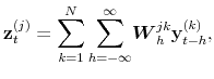
The filter output for each equals a sum of terms, each given by a weighting kernel applied to an element series. For , we will call the profile of weights an auto-filter, while for distinct indices they will be called a cross-filter, i.e., the weights for the signal are applied to a different series. We now have input series for each output series, so there are $N^{2}$ filters to consider.

The spectral representation for a stationary multivariate time series (see Chapter 11.6 of Brockwell and Davis (1991)) involves a vector-valued orthogonal increments process $d\mathbf{Z}(\lambda )$ for frequencies $% \lambda \in \lbrack -\pi ,\pi ]$ defined as $\mathbf{y}_{t} = \int_{-\pi }^{\pi } e^{it\lambda} \, d\mathbf{Z}(\lambda)$ . When this is well-defined, the spectral density matrix $\boldsymbol{F}$ is defined via $\mathbb{E }[ {% \vert d \mathbf{Z} (\lambda) \vert}^2 ]$ divided by $2 \pi$ , and describes the second moment variation in terms of power at different frequencies. The diagonal entries of $\boldsymbol{F}$ are the spectral densities of the component processes of $\{\mathbf{y}_{t}\}$ , whereas the off-diagonal entries are cross-spectral densities that summarize the relationships across series for the range of frequency parts. The output of the filter $\boldsymbol{W}(L)$ is expressed in the frequency domain as

$\displaystyle \mathbf{z}_{t}=\int_{-\pi }^{\pi }e^{it\lambda }\boldsymbol{W}(e^{-i\lambda })d\mathbf{Z}(\lambda ),$

(3)

with the quantity $\boldsymbol{W}(e^{-i\lambda })$ obtained by plugging the complex exponential into the filter formula (1); this gives the definition of the multivariate frequency response function (frf). That is, the frf $\boldsymbol{W}(e^{-i\lambda })$ is the discrete Fourier Transform (FT) of the weights sequence $\{ \boldsymbol{W}_{h} \}$ . A comparison of input and output in (3) indicates that the orthogonal increments process for $\{\mathbf{z}_{t}\}$ is $\boldsymbol{W}% (e^{-i\lambda })d\mathbf{Z}(\lambda )$ . Correspondingly, the spectral density matrix of the output process is $\boldsymbol{W}(e^{-i\lambda }) \boldsymbol{F} (\lambda) \boldsymbol{W}^{\prime }(e^{i\lambda }).$

For many filters of interest, including those we study in Section 4 below, $% \boldsymbol{W}_{-h}=\boldsymbol{W}_{h}$ for all , which implies the frf is real-valued. In this case there is no phase shift (see Brockwell and Davis (1991)) and the frf is identical with the Gain function, denoted $% \boldsymbol{G}$ , i.e., $\boldsymbol{G}(\lambda )=\boldsymbol{W}(e^{-i\lambda })$ . We focus on this case in what follows; if we examine the action for the th component output process, we have

$\displaystyle \mathbf{z}_{t}^{(j)}=\int_{-\pi }^{\pi }e^{it\lambda }\sum_{k=1}^{N}% \boldsymbol{W}^{jk}(e^{-i\lambda })d\mathbf{Z}_{k}(\lambda )=\sum_{k=1}^{N}\int_{-\pi }^{\pi }e^{it\lambda }\boldsymbol{G}^{jk}(\lambda )d\mathbf{Z}_{k}(\lambda ).$

So the gain is a

matrix-valued functions of frequency, whose

th components act to modulate the amplitude of variation for the contribution of the

th input series to the

th output series.

As noted above, the spectral density $\boldsymbol{F}$ gives a breakdown of the second order structure of a vector time series. An equivalent tool is the multivariate autocovariance generating function (ACGF), which for any mean zero stationary series $\boldsymbol{x}_{t}$ is written as

$\displaystyle \boldsymbol{\Gamma }_{\boldsymbol{x}}(L)=\overset{\infty }{\underset{% h=-\infty }{\sum }}\boldsymbol{\Gamma }_{h}L^{h},$

where $\boldsymbol{\Gamma }_{h}=E(\boldsymbol{x}_{t}\boldsymbol{x}% _{t-h}^{\prime })$ is the covariance between $\boldsymbol{x}_{t}$ and $% \boldsymbol{x}_{t-h}$ . Therefore, $\boldsymbol{\Gamma }_{\boldsymbol{x}% }(L)$ contains information about the autocovariances of each component of the vector process, as well as the cross-covariances of the various elements at different lags. The mapping from time to frequency domain, $\boldsymbol{F}% (\lambda )=\boldsymbol{\Gamma }_{\boldsymbol{x}}(e^{-i\lambda })$ , shows that the spectrum is the Fourier transform of the autocovariance sequence.

So far we have reviewed multivariate filters and properties of stationary vector time series. Now, the basic aim of signal extraction is to estimate a target signal $\boldsymbol{s}_{t}$ , in a series $\mathbf{y}_{t}$ of interest, or equivalently, to remove the remainder $\boldsymbol{n}_{t}$ , called the noise. A precise formulation is given by

$\displaystyle \mathbf{y}_{t}=\boldsymbol{s}_{t}+\boldsymbol{n}_{t}$

(4)

(for all $-\infty < t < \infty$ ), which assumes that the observed time series $\{\mathbf{y}_{t}\}$ can be decomposed into unobserved signal and noise, both of which have dimension $N\times 1$ . We also assume that $% \boldsymbol{s}_{t}$ and $\boldsymbol{n}_{t}$ are uncorrelated with one another, which is consistent with the large literature on signal extraction theory. The two component decomposition in (4) is actually a general formulation of signal extraction problems, because we can identify $\{\boldsymbol{s}_{t}\}$ with a particular component of interest or with an aggregate signal given by a sum of components, whereas $\{% \boldsymbol{n}_{t}\}$ consists of the sum of all the remaining parts of the observed time series.

The problem of multivariate signal extraction is to compute, for each and at each time , $\mathbb{E}[\mathbf{s}_{t}^{(j)}\vert\{\mathbf{y}_{t}\}]$ , the estimate that minimizes the Mean Squared Error (MSE) criterion. Interest centers on linear optimal estimators following Whittle (1963), as usually undertaken in the literature. The linear solution is, strictly speaking, only appropriate for Gaussian data. That is, the mean of the signal, conditional on the observations, is always given by a linear filter only under normality. For non-Gaussian data, the linear estimates constructed here do not yield the conditional expectation in all cases². However, for any type of white noise distribution, our linear estimators are still minimum MSE among all linear estimators.

In the case that both the signal and noise processes are stationary, the optimal filter for extracting the signal vector is

$\displaystyle \boldsymbol{W}_{WK}(L)=\boldsymbol{\Gamma }_{\boldsymbol{s}}(L)[\boldsymbol{% \Gamma }_{\boldsymbol{s}}(L)+\boldsymbol{\Gamma }_{\boldsymbol{n}}(L)]^{-1},$

(5)

where WK stands for the Wiener-Kolmogorov filter (see Wiener (1949); the formula under stationarity is also discussed more recently in Gómez (2006)). The filter for extracting the noise is $\boldsymbol{\Gamma }_{% \boldsymbol{n}}(L)[\boldsymbol{\Gamma }_{\boldsymbol{s}}(L)+\boldsymbol{% \Gamma }_{\boldsymbol{n}}(L)]^{-1}$ , which is $1_{N}-\boldsymbol{W}_{WK}(L)$ , where $1_{N}$ denotes an $N\times N$ identity matrix.

Now (5) gives the time-domain characterization, which when expressed in the form (1) shows the matrix weights applied to the series to extract the signal vector in a bi-infinite sample. To convert to the frequency domain, substitute $e^{-i\lambda }$ for , which then produces the WK frf:

$\displaystyle \boldsymbol{W}_{WK}(e^{-i\lambda })=\boldsymbol{\Gamma }_{\boldsymbol{s}% }(e^{-i\lambda })[\boldsymbol{\Gamma }_{\boldsymbol{s}}(e^{-i\lambda })+% \boldsymbol{\Gamma }_{\boldsymbol{n}}(e^{-i\lambda })]^{-1},$

where the quantities $\boldsymbol{\Gamma }_{\boldsymbol{s}}(e^{-i\lambda })$ and $\boldsymbol{\Gamma }_{\boldsymbol{n}}(e^{-i\lambda })$ are the multivariate spectral densities of signal and noise, respectively. Note that a multivariate WK filter's frf can have complex values, because the off-diagonal entries of $\boldsymbol{\Gamma }_{\boldsymbol{s}}(e^{-i\lambda })$ and $\boldsymbol{\Gamma }_{\boldsymbol{n}}(e^{-i\lambda })$ can be complex-valued when there is non-trivial phase shift between the components of the vector process.

Below, we extend this result to the nonstationary case, both under very general conditions on the component structure and under the similar specification form that usually holds for multivariate models used in research and applications, generalizing the classic results of Bell (1984). The first formulation involves detailed results allowing for a flexible form where the component design may differ across series. This would include, for instance, a situation where series have stochastic trends with different orders of integration. The second version refers to the uniform nonstationary operators form, often used in time series analysis, where the component orders of integration are the same across variables. Within this form, there are two possible portrayals: first, in terms of ACGFs of "over-differenced" signal and noise processes, $\mathbf{\partial u}$ and $% \mathbf{\partial v}$ defined below, in which case the stationarity of the processes immediately guarantees that the filter and its frf are well-defined; or second, explicitly in terms of signal and noise ACGFs (called pseudo-ACGFs when the component is nonstationary), which is directly analogous to (5) in terms of stationary ACGFs, in which case existence and convergence of the filter and its frf can be verified by taking appropriate limits.

For the multivariate signal and noise processes, we consider all processes that are difference-stationary: there is a "minimal" differencing operator (a polynomial in the lag operator that has all roots on the unit circle), and there is no way to factor the polynomial so that the remaining factors form an operator that by itself renders the process stationary. This includes openly formulated VARIMA specifications (see the discussion in Lütkepohl (2006) on integrated processes), or structural forms that involve intuitive restrictions (that help in model parsimony and interpretability).

We will use the term "core," to refer to the mean zero, covariance stationary process resulting from differencing. Note that the noise process may be nonstationary as well, but the differencing polynomials must be different from those of the signal process. This involves no loss of generality in practice; it is a simple requirement for keeping signal and noise well-defined. Components may also have co-integration or co-linearity, expressed as having a spectral density matrix for the core process that is singular at some (finite set of) frequencies.

Consider the th observed process, $\{\mathbf{y}_{t}^{(j)}\}$ . Since it is a difference-stationary process (e.g., VARIMA), by definition there exists an order $d^{j}$ polynomial $\delta ^{(j)}$ in the lag operator such that $\{\mathbf{w}_{t}^{(j)}\}=\{\delta ^{(j)}(L)\mathbf{y}_{t}^{(j)}\}$ is covariance stationary. Similarly, we suppose there are signal and noise differencing polynomials $\delta _{\mathbf{s}}^{(j)}$ and $\delta _{\mathbf{n}}^{(j)}$ that render each of them stationary, so that $\{\mathbf{u}% _{t}^{(j)}\}=\{\delta _{\mathbf{s}}^{(j)}(L)\mathbf{s}_{t}^{(j)}\}$ and $\{% \mathbf{v}_{t}^{(j)}\}=\{\delta _{\mathbf{n}}^{(j)}(L)\mathbf{n}_{t}^{(j)}\}$ . As a special and leading case, it may occur that the signal and noise differencing operators do not depend on , so that they are the same for each series (though they still differ for signal versus noise); we refer to this situation as "uniform differencing operators."

Let $\boldsymbol{F}_{\mathbf{u}}^{jk}$ , $\boldsymbol{F}_{\mathbf{v}}^{jk}$ , and $\boldsymbol{F}_{\mathbf{w}}^{jk}$ denote the cross-spectral density functions for the th and th processes for the signal, noise, and observed processes, respectively. These functions are the components of spectral matrices (which are functions of the frequency $\lambda$ ) denoted $% \boldsymbol{F}_{\mathbf{u}}$ , $\boldsymbol{F}_{\mathbf{v}}$ , and $% \boldsymbol{F}_{\mathbf{w}}$ . We suppose that $\boldsymbol{F}_{\mathbf{w}}$ is invertible almost everywhere, i.e., the set $\Lambda$ of frequencies where $\boldsymbol{F}_{\mathbf{w}}$ is noninvertible has Lebesgue measure zero. Note that if the data process is co-integrated (in the sense of Engle and Granger (1987)), then $\boldsymbol{F}_{\mathbf{w}} (0)$ is singular, but $\boldsymbol{F}_{\mathbf{w}} (\lambda)$ is invertible for $\lambda \neq 0$ . However (as shown below), if the innovations for $\{ \mathbf{w}_t \}$ are co-linear (i.e., the covariance of the white noise process has determinant zero) then $\boldsymbol{F}_{\mathbf{w}} (\lambda)$ is singular for all values of $\lambda$ , and our results don't apply - but neither is conventional model estimation possible. See the further discussion following Theorems 1 and 2. It is convenient to define the so-called "over-differenced" processes given by

$\displaystyle \partial \mathbf{u}_{t}^{(j)}$	$\displaystyle =\delta ^{(j)}(L)\mathbf{s}_{t}^{(j)}=\delta _{\mathbf{n}}^{(j)}(L)\mathbf{u}_{t}^{(j)}$
$\displaystyle \partial \mathbf{v}_{t}^{(j)}$	$\displaystyle =\delta ^{(j)}(L)\mathbf{n}_{t}^{(j)}=\delta _{\mathbf{s}}^{(j)}(L)\mathbf{v}_{t}^{(j)}.$

These occur when the full-differencing operator $\delta ^{(j)}(L)$ is applied to signal and noise respectively, resulting in covariance stationary processes that may have zeroes in their spectral densities.

Next, we assume that the vector processes $\{\mathbf{u}_{t}\}$ and $\{% \mathbf{v}_{t}\}$ are uncorrelated with one another. This is reasonable when signal and noise are driven by unrelated processes; for instance, the trend may be linked to long-run factors (like the setting of contracts), while the short-run run noise stems from temporary forces. The assumption of zero correlation also seems a natural choice when a correlation restriction is required for identification.

Note that each nonstationary process $\{\mathbf{y}_{t}^{(j)}\}$ can be generated from $d^{j}$ stochastic initial values $\mathbf{y}_{\ast }^{(j)}$ together with the disturbance process $\{\mathbf{w}_{t}^{(j)}\}$ , for each , in the manner elucidated for the univariate case in Bell (1984). The information contained in $\{\mathbf{y}_{t}^{(j)}\}$ is equivalent to that in $\{\mathbf{w}_{t}^{(j)}\}\cup \mathbf{y}_{\ast }^{(j)}$ for the purposes of linear projection, since the former is expressible as a linear transformation of the latter, for each . In model fitting and forecasting applications, a working assumption on vector time series is that these initial values $\mathbf{y}_{\ast }^{(j)}$ are uncorrelated with the disturbance process $\{\mathbf{w}_{t}^{(j)}\}$ ; we will assume a stronger condition that actually implies this assumption.

Assumption $M_{\infty }$ .

Suppose that, for each $j=1,2,\cdots ,N$ , the initial values $\mathbf{y}% _{\ast }^{(j)}$ are uncorrelated with the vector signal and noise core processes $\{\mathbf{u}_{t}\}$ and $\{\mathbf{v}_{t}\}$ .

This assumption generalizes the univariate Assumption A of Bell (1984) to a multivariate framework - each set of initial values $\mathbf{y}% _{\ast }^{(j)}$ are orthogonal not only to the signal and noise core processes for the th series, but for all series. Set $z=e^{-i\lambda }$ and $\overline{z}=e^{i\lambda }$ , and utilize the following notation, that for any matrix the matrix consisting of only the diagonal entries is written $\widetilde{A}$ . Then for nonstationary (and possibly co-integrated) multivariate time series, the optimal estimator of the signal, conditional on the observations $\{\mathbf{y}_{t}\}$ , for each and at each time , is given by a multivariate filter $\boldsymbol{W}(L)$ described below.

Theorem 1 Assume that $\boldsymbol{F}_{\mathbf{w}} (\lambda)$ is invertible for each $\lambda$ in a subset $\Lambda \subset [-\pi,\pi]$ of full Lebesgue measure. Also suppose that the vector processes $\{ \mathbf{u}% _t \}$ and $\{ \mathbf{v}_t \}$ are uncorrelated with one another, and that Assumption $M_{\infty }$ holds. Denote the cross-spectra between $\{ \mathbf{u}_t \}$ and $\{ \mathbf{w}_t \}$ via $\mathbf{\Gamma}_{\mathbf{u}, \mathbf{w}% } (z)$ , which has th entry $\boldsymbol{F}_{\mathbf{u}}^{jk} (\lambda) \delta_{\mathbf{n}}^{(k)} (\overline{z})$ . Similarly, denote the cross-spectra between $\{ \mathbf{v}_t \}$ and $\{ \mathbf{w}_t \}$ via $% \mathbf{\Gamma}_{\mathbf{v}, \mathbf{w}} (z)$ . Also, let $\widetilde{\mathbf{% \delta}} (z)$ denote the diagonal matrix with entries $\delta^{(j)} (z)$ . Consider the filter $\boldsymbol{W}(L)$ defined as follows: it has frf defined for all $\lambda \in \Lambda$ via the formula

$\displaystyle \boldsymbol{W} (z) = \widetilde{\mathbf{\Gamma}}_{\mathbf{w}}^{-1} (z) \left[ \widetilde{\mathbf{\Gamma}}_{\partial \mathbf{u}} (z) - \left( \widetilde{% \mathbf{\Gamma}}_{\mathbf{u}, \mathbf{w}}(z) \mathbf{\Gamma}_{\mathbf{v}, \mathbf{w}} (z) - \widetilde{\mathbf{\Gamma}}_{\mathbf{v}, \mathbf{w}}(z) \mathbf{\Gamma}_{\mathbf{u}, \mathbf{w}} (z) \right) \mathbf{\Gamma}_{% \mathbf{w}}^{-1} (z) \, \widetilde{\mathbf{\delta}} (z) \right].$

(6)

Moreover, we suppose that this formula can be continuously extended to $% \lambda \not\in \Lambda$ , and we refer to this extension by $\boldsymbol{W} (z)$ as well. Then the optimal estimate of the signal at time

is given by $\widehat{\mathbf{s}}_t = \boldsymbol{W} (L) \mathbf{y}_t$ . Let $% \widetilde{\mathbf{\Gamma}}_{\mathbf{u}, \mathbf{w}} (z) \mathbf{\Gamma}_{% \mathbf{v}, \mathbf{w}} (z) - \widetilde{\mathbf{\Gamma}}_{\mathbf{v}, \mathbf{w}} (z)\mathbf{\Gamma}_{\mathbf{u}, \mathbf{w}} (z)$ be abbreviated by $\mathbf{B}(z)$ . Then the spectral density of the signal extraction error process is given by

	$\displaystyle \widetilde{\mathbf{\Gamma}}_{\mathbf{w}}^{-1} (z) \widetilde{\mathbf{\Gamma }}_{\mathbf{u}, \mathbf{w}} (z) \boldsymbol{F}_{\mathbf{v}} (\lambda) \widetilde{\mathbf{\Gamma}}_{\mathbf{u}, \mathbf{w}}^{\prime} (\overline{z}) \widetilde{\mathbf{\Gamma}}_{\mathbf{w}}^{-1} (z) + \widetilde{\mathbf{\Gamma }}_{\mathbf{w}}^{-1} (z) \widetilde{\mathbf{\Gamma}}_{\mathbf{v}, \mathbf{w}% } (z) \boldsymbol{F}_{\mathbf{u}} (\lambda) \widetilde{\mathbf{\Gamma}}_{% \mathbf{v}, \mathbf{w}}^{\prime} (\overline{z}) \widetilde{\mathbf{\Gamma}}_{% \mathbf{w}}^{-1} (z)$
	$\displaystyle - \widetilde{\mathbf{\Gamma}}_{\mathbf{w}}^{-1} (z) \mathbf{B}(z) \mathbf{% \Gamma}_{\mathbf{w}}^{-1} (z) \mathbf{B}^{\prime}(\overline{z}) \widetilde{% \mathbf{\Gamma}}_{\mathbf{w}}^{-1} (z).$

When the differencing operators are uniform, a compact matrix formula for $% \boldsymbol{F} (z)$ is given by

$\displaystyle \boldsymbol{F} (z)= \mathbf{\Gamma}_{ \partial \mathbf{u} } (z ) \mathbf{% \Gamma}_{\mathbf{w}}^{-1} (z) = \boldsymbol{F}_{\partial \mathbf{u} } (\lambda) \, \boldsymbol{F}_{ \mathbf{w}}^{-1} (\lambda)$

(7)

for $\lambda \in \Lambda$ , and by the limit of such for $\lambda \not\in \Lambda$ ; the error spectral density is $\mathbf{\ \Gamma}_{\mathbf{u}} (z) \mathbf{\Gamma}_{\mathbf{w}}^{-1} (z) \mathbf{\Gamma}_{\mathbf{v}} (z)$ .

Remark 1 Because $\mathbf{\Gamma}_{\mathbf{w}} = \mathbf{\Gamma}_{\partial \mathbf{u}} + \mathbf{\Gamma}_{\partial \mathbf{v}}$ , (7) generalizes (5) to the nonstationary case. If some of the differencing polynomials are unity (i.e., no differencing is required to produce a stationary series), the formula collapses down to the classical case. In the extreme case that all the series are stationary, trivially $\partial \mathbf{u}_{t}=\mathbf{s}_{t}$ and $\partial \mathbf{v}_{t}=\mathbf{n}_{t}$ for all times . The second expression for the frf in (7) shows how this is a direct multivariate generalization of the univariate frf in Bell (1984), which has the formula ${\vert\delta _{n}(z)\vert}^{2}f_{u}(\lambda )/f_{w}(\lambda )$ .

Theorem 1 is worded so as to include the important case of co-integrated vector time series (Engle and Granger, 1987), as $\boldsymbol{F}_{\mathbf{w}}$ is only required to be invertible at most frequencies. We next show that the key assumptions of Theorem 1 on the structure of $\boldsymbol{W} (z)$ are satisfied for a very wide class of co-integrated processes. We present our discussion in the context of uniform differencing operators - a result can be formulated for the more general case, but it is much more difficult to state, and the uniform differencing operator situation is sufficient for most, if not all, econometric applications of interest.

The vector signal and noise processes satisfy $\delta _{\mathbf{s}}(L)% \mathbf{s}_{t}=\mathbf{u}_{t}$ and $\delta _{\mathbf{n}}(L)\mathbf{n}_{t}=% \mathbf{v}_{t}$ , and we suppose that a Wold decomposition can be found for these core processes:

$\displaystyle \mathbf{u}_{t}=\Xi (L)\mathbf{\zeta }_{t}\qquad \mathbf{v}_{t}=\Omega (L)% \mathbf{\kappa }_{t},$

(8)

where $\{\mathbf{\zeta }_{t}\}$ and $\{\mathbf{\kappa }_{t}\}$ are uncorrelated multivariate white noise processes. The MA filters $\Xi (z)$ and $\Omega (z)$ are linear and causal by assumption, and we assume that the white noise covariance matrices $\Sigma _{\mathbf{\zeta }}$ and $\Sigma _{% \mathbf{\kappa }}$ are non-negative definite. Then $\boldsymbol{F}_{\mathbf{u}} (\lambda) = \Xi (z) \Sigma _{\mathbf{\zeta }} \Xi^{\prime} (\overline{z})$ , which is singular (for a given $\lambda$ ) iff either $\vert\Sigma _{\mathbf{% \zeta }}\vert = 0$ or there exists a matrix

(depending on $\lambda$ ) such that $a^{\prime} \Xi (z) = 0$ . The former case is described as co-linearity of the innovations, or in particular is referred to as "common trends" when the signal is a trend (see Stock and Watson (1988)). The latter case is a type of co-integration (with

the co-integrating relations), although more properly the term is only applied when $a^{\prime} \Psi (1) = 0$ , i.e., there is a singularity at the $\lambda = 0$ frequency. Singularities in the spectrum of a core process can only arise in one of these two ways, as co-linearity or co-integration (in our generalized sense). Moreover, in the former case it must follow that the spectrum is singular at all frequencies, whereas in the latter case there could be an isolated number of singular matrices.

In order that the data core spectrum $\boldsymbol{F}_{\mathbf{w}}$ is invertible almost everywhere, it is convenient to assume that $\boldsymbol{F}% _{\mathbf{v}}$ is positive definite at all frequencies; as shown below, this is a sufficient condition. Such a noise core process is said to be invertible, by definition.

Proposition 1 Suppose that the differencing operators are uniform and that the core processes follow (8). Also suppose that $\mathbf{v}_t$ is invertible. Then $\boldsymbol{F_{w}}$ is invertible except at a finite set of frequencies, and $\boldsymbol{W} (z)$ defined in (7) can be continuously extended from its natural domain $\Lambda$ to all of $[-\pi,\pi]$ .

The argument also works with the roles of signal and noise swapped; we require that one of the core component processes be invertible. So the formula for the WK frf is well-defined - by taking the appropriate limits at the nonstationary frequencies - and (7) can be used to give a compact expression for the filter, formally substituting for $z=e^{-i\lambda }$ :

$\displaystyle \boldsymbol{W} (L)=\mathbf{\Gamma}_{\partial \mathbf{u}}(L){\ \left[ \mathbf{% \Gamma}_{\partial \mathbf{u}}(L)+\mathbf{\Gamma}_{\partial \mathbf{v}}(L)% \right] }^{-1}.$

(9)

This expresses the filter in terms of the ACGFs of the over-differenced signal and noise processes.

We can re-express this in terms of the so-called pseudo-ACGFs of signal and noise, which are defined via

$\displaystyle \mathbf{\Gamma }_{\mathbf{s}}(L)=\mathbf{\Gamma }_{\mathbf{u}}(L){\ \left[ \widetilde{\delta }_{\mathbf{s}}(L)\widetilde{\delta }_{\mathbf{s}}(L^{-1})% \right] }^{-1}\qquad \mathbf{\Gamma }_{\mathbf{n}}(L)=\mathbf{\Gamma }_{% \mathbf{v}}(L){\ \left[ \widetilde{\delta }_{\mathbf{n}}(L)\widetilde{\delta }_{\mathbf{n}}(L^{-1})\right] }^{-1}.$

As usual, the tilde denotes a diagonal matrix; here the entries correspond to the differencing polynomials for each series. This generalizes the ACGF structure from stationary to nonstationary multivariate processes. Also $% \mathbf{\Gamma }_{\partial \mathbf{u}}(L)=\mathbf{\Gamma }_{\mathbf{s}}(L)% \widetilde{\mathbf{\delta }}(L)\widetilde{\mathbf{\delta }}(L^{-1})$ and $% \mathbf{\Gamma }_{\partial \mathbf{v}}(L)=\mathbf{\Gamma }_{\mathbf{n}}(L)% \widetilde{\mathbf{\delta }}(L)\widetilde{\mathbf{\delta }}(L^{-1})$ , so that when the differencing operators are uniform (9) reduces to (5). Even though $\mathbf{\Gamma }_{\mathbf{s}% }(L)$ and $\mathbf{\Gamma }_{\mathbf{n}}(L)$ are not strictly well-defined by themselves, as the infinite series representing their ACGF may not converge, the cancellations that occur ensure that $\boldsymbol{W}(L)$ is indeed well-defined. Note that it was not obvious at the outset that (5) would hold with pseudo-ACGFs replacing the ACGFs of the stationary case; the steps in the proof are crucial for verifying the form of the filter from the differencing operators and core stationary processes. With (5) confirmed to hold generally, we can directly form filters for the nonstationary models of interest for multiple economic series.

Whereas in the univariate case one can compute filter coefficients readily from the filter formula (9) - by identifying the frf as the spectral density of an associated ARMA process and using standard inverse FT algorithms - the situation is more challenging in the multivariate case. Instead, coefficients would be determined by numerical integration. Although this may be done, for practical applications we rather recommend the exact finite sample approach of the next section. Of course, filters can be expressed for both signal and noise extraction, and trivially by (7) the sum of their respective frfs is the identity matrix (as a function of $\lambda$ ). This is analogous to the univariate case, where signal and noise frfs sum to unity for all $\lambda$ .

3 Multivariate signal extraction from a finite sample

We now discuss multivariate signal extraction for a finite sample from a time series, and present exact matrix formulas for the solution to the problem. This represents the first treatment of the multivariate case for either the stationary or nonstationary frameworks. Even away from the end-points in a relatively long but finite sample, there is a certain attraction to having the unique optimum signal derived from the underlying theory. However, the main interest for applications like current monitoring of price trends lies in estimators near the end of series, for which the formulas give an analytical characterization and reveal the explicit dependence on series' individual parameters, on cross-relationships, and on sample size and signal location.

As in Section 2, we consider time series $\{\mathbf{y}_{t}^{(j)}\}$ for $% 1\leq j\leq N$ , and suppose that each series can be written as the sum of unobserved signal and noise components, denoted $\{\mathbf{s}_{t}^{(j)}\}$ and $\{\mathbf{n}_{t}^{(j)}\}$ , such that (4) holds for all . While in the previous section, we considered unbounded in both directions, here we suppose the time range of the sample consists of $% t=1,2,\cdots ,T$ . We will express the realizations of each series as a length- vector, namely $\mathbf{y}^{(j)}={ [y_{1}^{(j)},y_{2}^{(j)},...,y_{T}^{(j)}]}^{\prime }$ , and similarly for signal, $\mathbf{s}^{(j)},$ and noise, $\mathbf{n}^{(j)}$ . For each , the optimal estimate is the conditional expectation $\mathbb{E}[\mathbf{s}^{(j)}\vert% \mathbf{y}^{(1)},\mathbf{y}^{(2)},\cdots ,\mathbf{y}^{(N)}]$ . As in the previous section, the definition of optimality used here is the minimum MSE estimator under normality and the best linear estimator with non-Gaussian specifications.

So our estimate $\widehat{\mathbf{s}}^{(j)}$ can be expressed as a $T\times (NT)$ matrix acting on all the data vectors stacked up, or equivalently as

$\displaystyle \widehat{\mathbf{s}}^{(j)}=\sum_{k=1}^{N}F^{jk}\mathbf{y}^{(k)}.$

Each matrix $F^{jk}$ is $T\times T$ dimensional. The notation here is as follows: the first superscript is associated with the output

, whereas the second superscript is associated with the input

. Our task is to compute the entries of $F^{jk}$ such that error process $\widehat{\mathbf{s}}% ^{(j)}-\mathbf{s}^{(j)}$ is uncorrelated with the observed data. As shown below, the coefficients of $F^{jk}$ depend heavily on the properties of the Data Generating Processes (DGPs) for signal and noise. As in the previous section, our treatment encompasses any general signal and noise (for each

, $\delta _{\mathbf{s}}^{(j)}$ and $\delta _{\mathbf{n}}^{(j)}$ are composed of fully distinct factors) processes with nonstationary operators that may differ across series.

We may express the specification of the finite series in matrix notation with $\Delta ^{(j)}\mathbf{y}^{(j)}$ being a stationary vector, where $% \Delta ^{(j)}$ is a $T-d^{j}\times T$ dimensional matrix whose rows consist of the coefficients of $\delta ^{(j)}$ , appropriately shifted. (For the treatment of the univariate case, see McElroy (2008).) The application of each $\Delta ^{(j)}$ yields a stationary vector, called $\mathbf{w}^{(j)}$ , which has length $T-d^{j}$ (so $\mathbf{w}^{(j)}={\ [\mathbf{w}% _{d^{j}+1}^{(J)},\cdots ,\mathbf{w}_{T}^{(j)}]}^{\prime }$ ). These vectors may be correlated with one another and among themselves, which is summarized in the notation $\mathbb{E}[\mathbf{w}^{(j)}{\mathbf{w}^{(k)}}^{\prime }]=\Sigma _{\mathbf{w}}^{jk}$ . We further suppose that the differencing is taken such that all random vectors have mean zero (this presupposes that fixed effects have been removed via regression). Note that this definition includes processes that are nonstationary only in second moments, i.e., heteroskedastic. Therefore, the setup is somewhat broader than in the previous section where the core processes were assumed covariance stationary.

This discussion can also be extended to the signal and noise components as follows. We form the matrices $\Delta _{\mathbf{s}}^{(j)}$ and $\Delta _{% \mathbf{n}}^{(j)}$ corresponding to the signal and noise differencing polynomials $\delta _{\mathbf{s}}^{(j)}$ and $\delta _{\mathbf{n}}^{(j)}.$ Let $\mathbf{u}^{(j)}=\Delta _{\mathbf{s}}^{(j)}\mathbf{s}^{(j)}$ and $% \mathbf{v}^{(j)}=\Delta _{\mathbf{n}}^{(j)}\mathbf{n}^{(j)}$ , with cross-covariance matrices denoted $\Sigma _{\mathbf{u}}^{jk}$ and $\Sigma _{% \mathbf{v}}^{jk}$ . Now assume there are no common roots among $\delta _{% \mathbf{s}}^{(j)}$ and $\delta _{\mathbf{n}}^{(j)}$ , so that $\delta ^{(j)}(L)=\delta _{\mathbf{s}}^{(j)}(L)\delta _{\mathbf{n}}^{(j)}(L)$ . Then as in the univariate case (McElroy and Sutcliffe, 2006), we have

$\displaystyle \Delta ^{(j)}=\underline{\Delta }_{\mathbf{n}}^{(j)}\Delta _{\mathbf{s}% }^{(j)}=\underline{\Delta }_{\mathbf{s}}^{(j)}\Delta _{\mathbf{n}}^{(j)},$

(10)

where $\underline{\Delta }_{\mathbf{n}}^{(j)}$ and $\underline{\Delta }_{% \mathbf{s}}^{(j)}$ are similar differencing matrices of reduced dimension, having $T-d^{j}$ rows. It follows that

$\displaystyle \mathbf{w}^{(j)}=\Delta ^{(j)}\mathbf{y}^{(j)}=\underline{\Delta }_{\mathbf{n}}^{(j)}\mathbf{u}^{(j)}+\underline{\Delta }_{\mathbf{s}}^{(j)}\mathbf{v}% ^{(j)},$

(11)

and hence - if $\mathbf{u}^{(j)}$ and $\mathbf{v}^{(k)}$ are uncorrelated for all

$\displaystyle \Sigma _{\mathbf{w}}^{jk}=\underline{\Delta }_{\mathbf{n}}^{(j)}\Sigma _{% \mathbf{u}}^{jk}{\underline{\Delta }_{\mathbf{n}}^{(k)}}^{\prime }+% \underline{\Delta }_{\mathbf{s}}^{(j)}\Sigma _{\mathbf{v}}^{jk}{\underline{% \Delta }_{\mathbf{s}}^{(k)}}^{\prime }.$

We can splice all these $\Sigma _{\mathbf{w}}^{jk}$ matrices together as block matrices in one large matrix $\Sigma _{\mathbf{w}}$ , which is also the covariance matrix of $\mathbf{w}$ , the vector composed by stacking all the $% \mathbf{w}^{(j)}$ . A key condition for optimal filtering is the invertibility of $\Sigma _{\mathbf{w}}$ . Further, the Gaussian likelihood function for the differenced sample involves the quadratic form $\mathbf{w}% ^{\prime }\Sigma _{\mathbf{w}}^{-1}\mathbf{w}$ , so parameter estimation on this basis also requires an invertible covariance matrix. Below, we show that for possibly co-linear signal-noise decompositions and homoskedastic core processes, the invertibility of $\Sigma _{\mathbf{w}}$ is guaranteed.

Up to this point, we have set out notation and some basic working assumptions. For the signal extraction formula below, we require a few additional assumptions: let $\Sigma _{\mathbf{u}}^{jj}$ and $\Sigma _{% \mathbf{v}}^{jj}$ be invertible matrices for each , assume that $\mathbf{u}^{(j)}$ and $\mathbf{v}^{(k)}$ are uncorrelated with one another for all , and suppose that the initial values of $\mathbf{y}^{(j)}$ are uncorrelated with $\mathbf{u}^{(k)}$ and $\mathbf{v}^{(k)}$ for all . These initial values consist of all the first $d^{j}$ values of each sampled series $\mathbf{y}^{(j)}$ . This type of assumption is less stringent than $% M_{\infty }$ of the previous subsection, and will be called Assumption $% M_{T}$ instead.

Assumption .

Suppose that, for each $j=1,2,\cdots ,N$ , the initial values of $\mathbf{y}% ^{(j)}$ (the first $d^{j}$ observations) are uncorrelated with $\mathbf{u}$ and $\mathbf{v}$ .

Since Assumption $M_{T}$ entails that the initial values of the observed process are uncorrelated with $\mathbf{w}$ , it implies the condition often used to give a relatively simple Gaussian likelihood. Our main result below involves block matrices, and we use the following notation. If is a block matrix partitioned into sub-matrices $G^{jk}$ , then $\widetilde{G}$ denotes a block matrix consisting of only the diagonal sub-matrices $G^{jj}$ , being zero elsewhere.

Theorem 2 Assume that $\Sigma _{\mathbf{w}}$ is invertible, along with all $\Sigma _{\mathbf{u}}^{jj}$ and $\Sigma_{\mathbf{v}}^{jj}$ matrices, and that $\mathbf{u}^{(j)}$ and $\mathbf{v}^{(k)}$ are uncorrelated with one another for all and . Also suppose that Assumption holds. Let

$\displaystyle M^{jj}={\Delta _{\mathbf{n}}^{(j)}}^{\prime }{\Sigma _{\mathbf{v}}^{jj}}% ^{-1}\Delta _{\mathbf{n}}^{(j)}+{\Delta _{\mathbf{s}}^{(j)}}^{\prime }{% \Sigma _{\mathbf{u}}^{jj}}^{-1}\Delta _{\mathbf{s}}^{(j)}.$

Then $M^{jj}$ is invertible. If $\widehat{\mathbf{s}} = F \mathbf{y}$ is the optimal estimate of the signal, then the matrix

is defined as follows. Letting $\Psi _{\mathbf{w}}=\Sigma _{\mathbf{w}}^{-1}$ , we have

$\displaystyle F^{jj}$	$\displaystyle ={\ M^{jj}}^{-1}\left[ {\Delta _{\mathbf{n}}^{(j)}}^{\prime }{\Sigma _{\mathbf{v}}^{jj}}^{-1}\Delta _{\mathbf{n}}^{(j)}+\Sigma _{\ell \neq j}\left( {\Delta _{\mathbf{s}}^{(j)}}^{\prime }{\Sigma _{\mathbf{u}}^{jj}}% ^{-1}\Sigma _{\mathbf{u}}^{j \ell}{\ \underline{\Delta }_{\mathbf{n}% }^{(\ell)}}^{\prime }-{\Delta _{\mathbf{n}}^{(j)}}^{\prime }{\Sigma _{% \mathbf{v}}^{jj}}^{-1}\Sigma _{\mathbf{v}}^{j \ell}{\underline{\Delta }_{% \mathbf{s}}^{(\ell)}}^{\prime }\right) \Psi _{\mathbf{w}}^{\ell j}\Delta ^{(j)}\right]$
$\displaystyle F^{jk}$	$\displaystyle ={\ M^{jj}}^{-1}\Sigma _{\ell =1}^{N}\left( {\Delta _{\mathbf{s}% }^{(j)}}^{\prime }{\Sigma _{\mathbf{u}}^{jj}}^{-1}\Sigma _{\mathbf{u}}^{j \ell}{\underline{\Delta }_{\mathbf{n}}^{(\ell)}}^{\prime }-{\Delta _{\mathbf{% n}}^{(j)}}^{\prime }{\Sigma _{\mathbf{v}}^{jj}}^{-1}\Sigma _{\mathbf{v}}^{j \ell}{\underline{\Delta }_{\mathbf{s}}^{(\ell)}}^{\prime }\right) \Psi _{% \mathbf{w}}^{\ell k}\Delta ^{(k)}$

for $j\neq k$ . The signal extraction covariance matrix between the

th and

th error vectors is given by ${M^{jj}}^{-1}V^{jk}{M^{kk}}^{-1}$ , where $% V^{jk}$ is given by

	$\displaystyle \sum_{\ell,m=1}^{N}\left[ {\ \Delta _{\mathbf{n}}^{(j)}}^{\prime ... ...hbf{v}}^{mk}{\Sigma _{\mathbf{v}}^{kk}}% ^{-1}\Delta _{\mathbf{n}}^{(k)}\right]$
	$\displaystyle +{\ \Delta _{\mathbf{n}}^{(j)}}^{\prime }{\Sigma _{\mathbf{v}}^{jj}}% ^{-1}\Sigma _{\mathbf{v}}^{jk}{\Sigma _{\mathbf{v}}^{kk}}^{-1}\Delta _{% \mathbf{n}}^{(k)}+{\ \Delta _{\mathbf{s}}^{(j)}}^{\prime }{\Sigma _{\mathbf{u}}^{jj}}^{-1}\Sigma _{\mathbf{u}}^{jk}{\Sigma _{\mathbf{u}}^{kk}}^{-1}\Delta _{\mathbf{s}}^{(k)}.$

A compact matrix formula for

is given as follows. Define block-matrices

that have

th block matrix entries given, respectively, by

$\displaystyle A^{jk}$	$\displaystyle = {\ \Delta_{\mathbf{s}}^{(j)}}^{\prime} {\Sigma_{\mathbf{u}}^{jj}}% ^{-1} \Sigma_{\mathbf{u}}^{jk} {\Sigma_{\mathbf{u}}^{kk} }^{-1} \Delta_{% \mathbf{s}}^{(k)}$
$\displaystyle B^{jk}$	$\displaystyle = {\ \Delta_{\mathbf{n}}^{(j)}}^{\prime} {\Sigma_{\mathbf{v}}^{jj}}% ^{-1} \Sigma_{\mathbf{v}}^{jk} {\Sigma_{\mathbf{v}}^{kk} }^{-1} \Delta_{% \mathbf{n}}^{(k)}$
$\displaystyle C^{jk}$	$\displaystyle = {\ \Delta_{\mathbf{s}}^{(j)}}^{\prime} {\Sigma_{\mathbf{u}}^{jj}}% ^{-1} \Sigma_{\mathbf{u}}^{jk} {\underline{\Delta}_{\mathbf{n}}^{(k)}}% ^{\prime}$
$\displaystyle D^{jk}$	$\displaystyle = {\ \Delta_{\mathbf{n}}^{(j)}}^{\prime} {\Sigma_{\mathbf{v}}^{jj}}% ^{-1} \Sigma_{\mathbf{v}}^{jk} {\underline{\Delta}_{\mathbf{s}}^{(k)}}% ^{\prime}.$

Also let $\widetilde{\Delta}$ denote a block diagonal matrix with the matrix $\Delta ^{(j)}$ in the

th diagonal. Then

$\displaystyle M$	$\displaystyle = \widetilde{A} + \widetilde{B}$
$\displaystyle F$	$\displaystyle = M^{-1} \left[ \widetilde{B} + \left( C - D \right) \Sigma_{\mathbf{w}% }^{-1} \widetilde{\Delta} \right]$
$\displaystyle V$	$\displaystyle = A + B + (C - D) \Sigma_{\mathbf{w}}^{-1} {(C - D)}^{\prime},$

and the covariance matrix of the error vector is $M^{-1} V M^{-1}$ .

Remark 2 These formulas tell us mathematically how each series $\mathbf{y}% ^{(k)}$ contributes to the component estimate $\widehat{\mathbf{s}}^{(j)}$ . From the formulas for $F^{jj}$ and $F^{jk}$ we see that only the noise in $% \mathbf{y}^{(j)}$ is differenced, while for all other series both signal and noise are differenced. When there is no cross-series information, i.e., $% \Sigma _{\mathbf{u}}^{jk}$ and $\Sigma _{\mathbf{v}}^{jk}$ are zero for $% j\neq k$ , then clearly and are zero, and reduces to an -fold stacking of the univariate filter ( $M^{-1}\widetilde{B}$ is just the stacking of the univariate matrix filters of McElroy (2008)).

The matrix formula for is predicated on a specific way of stacking the time series data into $\mathbf{y}$ . This is a particularly convenient form, since each sub-matrix $F^{jk}$ can be easily peeled off from the block matrix , and directly corresponds to the contribution of the th series to the signal estimate for the th series. Stacking the data in another order - e.g., with all the observations for time together, followed by , etc. - would scramble the intuitive structure in .

In particular, one may pass to this alternative stacking, written as

$\displaystyle \mathbf{w}^{\flat }={[w_{1}^{(1)},w_{1}^{(2)},\cdots ,w_{1}^{(N)},w_{2}^{(1)},w_{2}^{(2)},\cdots ,w_{2}^{(N)},\cdots ]}^{\prime },$

via application of a $NT\times NT$ dimensional permutation matrix

. This format is more typical for describing VARMA processes, for example (see Lütkepohl (2006)). The covariance matrix of $\Sigma _{\mathbf{w}^{\flat }}$ has a familiar form, being block-Toeplitz with

th block $\mathbf{\Gamma }% _{j-k}$ , the acf of $\{\mathbf{w}_{t}\}$ . Of course, $\Sigma _{\mathbf{w}% }=P^{-1}\Sigma _{\mathbf{w}^{\flat }}P^{-1 \prime}$ , so invertibility of the one form is equivalent to invertibility of the other.

Let us consider any length column vector (which may be stochastic or deterministic), consisting of subvectors of length , where $% t=1,2,\cdots ,T$ . Then

$\displaystyle x^{\prime} \Sigma_{\mathbf{w}^{\flat}} x = \sum_{t,s} x_t^{\prime} \mathbf{% \Gamma}_{t-s} x_s = \frac{1}{2 \pi} \int_{-\pi}^{\pi} x^{\prime} (-\lambda) \mathbf{F}_{\mathbf{w}} (\lambda) x (\lambda) \, d\lambda,$

where $x(\lambda) = \sum_{t=1}^T x_t e^{-i \lambda t}$ . Now in the case that the signal is co-linear (but the noise is not), there exist a finite set of frequencies $\{ \lambda_s \}$ such that $\mathbf{F}_{\mathbf{w}} (\lambda_s)$ is not positive definite - see Proposition 2 and its proof for additional details. Hence it is possible to select $x_{\lambda_s}$ - corresponding to this frequency $\lambda_s$ - such that $% x_{\lambda_s}^{\prime} (-\lambda) \mathbf{F}_{\mathbf{w}} (\lambda) x_{\lambda_s} (\lambda)$ is zero when evaluated at this $\lambda_s$ frequency. However, the integrand above will be nonzero at all other frequencies; hence $\Sigma _{\mathbf{w}^{\flat }}$ is positive definite, and therefore invertible. If on the other hand the innovations of $\{ \mathbf{w}% _t \}$ were co-linear, a similar argument shows that $\mathbf{F}_{\mathbf{w}% } (\lambda)$ is singular for all $\lambda$ , and hence $\Sigma _{\mathbf{w}}$ would be singular.

But $\Sigma _{\mathbf{w}}$ is invertible for processes consisting of co-linear core signal and invertible core noise (or vice versa), which indicates that maximum likelihood estimation is viable; the Gaussian log likelihood is

$\displaystyle \log L(\mathbf{w,}\Sigma _{\mathbf{w}})= - \, (\mathbf{w}^{\prime }\Sigma _{% \mathbf{w}}^{-1}\mathbf{w}+\log \vert\Sigma _{\mathbf{w}}\vert)/2,$

(12)

up to a constant irrelevant for maximization (once we factor out the initial value vectors using Assumption $M_{T}$ ). It is interesting that the Whittle likelihood is not well-defined when $\mathbf{F}_{\mathbf{w}}$ has zeroes, as alluded to in the proof of Proposition 2.

The use of these formulas have some advantages over the state space approach. Certain questions, which involve the covariances of the signal extraction error across different time points, can be directly addressed with a matrix analytical approach. Also, the expressions are of practical interest when processes cannot be embedded in State Space Form (SSF); for example, a long memory cannot be cast in this form without truncation, which radically alters the memory dynamics. Generally, so long as the covariance and cross-covariance matrices used in Theorem 3 are available, the results apply. So we may consider heteroskedastic core processes and see the exact functional dependence of the filters on each time-varying variance parameter.

Furthermore, we can estimate any linear function of the signal. Supposing that our quantity of interest is $H\mathbf{s}$ for some large matrix applied to the stacked signal vector $\mathbf{s}$ (for example, $H\mathbf{s}$ could be the rate of change of the signal processes), then the optimal estimate for this quantity is simply $HF\mathbf{y}$ by the linearity of the conditional expectation (for Gaussian time series). Also, since the error covariance matrix for the estimation of $\mathbf{s}$ is $M^{-1} V M^{-1}$ , it follows that the error covariance matrix (whose diagonals are the MSEs) for our estimate of $H\mathbf{s}$ is $HM^{-1}VM^{-1}VH^{\prime }$ . Thus, for non-trivial problems a full knowledge of all the entries of and is required.

One particular case that is simple and of practical interest arises when is composed of unit vectors such that $H\mathbf{s}=\mathbf{s}^{(j)}$ . That is, we are interested in the th component of the signal at all sampled time points. Since $\mathbf{s}^{(j)}$ is just a projection of $\mathbf{s}$ , its extraction matrix is given by the same projection applied to . So the components of the optimal signal estimate are equal to the optimal estimates of the components of the signal (by linearity of conditional expectations).

4 Signal extraction for related and common trends

We now use the general results of Sections 2 and 3 to treat a few stochastic trend models widely used in econometrics. After reviewing these models, we develop the corresponding signal extraction filters, discussing some of the new, key aspects of the multivariate nonstationary case that warrant special attention.

4.1 Discussion of models

Since many economic time series are subject to permanent changes in level, there has been extensive research on models with stochastic trends. Models with related trends, where the underlying permanent shocks are correlated, allow us to establish links between series in their long-run behavior.

When there exists a particularly close relationship in the long-run movements across variables, as when series are co-integrated, there are some special implications for trend extraction, as we discuss later. A natural way to think about co-integration is in terms of common trends (i.e., co-linear innovations), as in Stock and Watson (1988) and Harvey (1989). A co-integrating relationship implies a tight long-run connection between a set of variables, with any short-run deviations in the relationships tending to correct themselves as time passes. Then, the long-run components of different series move together in a certain sense (there exist linear combinations of the trends that fluctuate around zero, i.e., are stationary). In the case of common trends, as demonstrated in the next sub-section, the gain functions for signal extraction have a collective structure at the frequency origin. Otherwise, in the absence of commonality, no matter how closely related the trends are, the filters decouple at the zero frequency.

As in the treatment given in Nyblom and Harvey (2000), we define the vector process $\boldsymbol{\mu }_{t}=(\mu _{t}^{(1)},...,$ $\mu _{t}^{(N)})^{\prime }$ as the trend, $\boldsymbol{\varepsilon }% _{t}=(\varepsilon _{t}^{(1)},...,$ $\mathbf{\varepsilon}_{t}^{(N)})^{\prime }$ as the irregular, and $\mathbf{y}_{t}=(y_{t}^{(1)},...,$ $% y_{t}^{(N)})^{\prime }$ as the observed series. Then the multivariate Local Level Model (LLM) is given by

$\displaystyle \mathbf{y}_{t}$	$\displaystyle =$	$\displaystyle \boldsymbol{\mu }_{t} + \boldsymbol{\varepsilon}_{t}, \qquad \quad \boldsymbol{\varepsilon}_{t} \sim WN(0,\boldsymbol{\Sigma }% _{\varepsilon })$	(13)
$\displaystyle \boldsymbol{\mu }_{t}$	$\displaystyle =$	$\displaystyle \boldsymbol{\mu}_{t-1} + \boldsymbol{\eta }_{t}, \quad \boldsymbol{\eta }_{t} \sim WN(0,\boldsymbol{\Sigma }_{\eta })$

where $WN(0,\boldsymbol{\Sigma })$ denotes that the vector is white noise, i.e., serially uncorrelated with zero mean vector and $N\times N$ non-negative definite covariance matrix $\mathbf{\Sigma }$ ; note that we may allow $\vert\mathbf{\Sigma }\vert = 0$ , which means that the innovations are co-linear. The irregular $\{ \boldsymbol{\varepsilon}_t \}$ accounts for transient factors, for instance, short-run movements due to weather, and is assumed to be invertible. However, the trend innovations $\{ \boldsymbol{% \eta }_{t} \}$ are possibly co-linear, which is equivalent to saying that $% \boldsymbol{\Sigma }_{\eta }$ may have reduced rank

. When this occurs, we can rewrite (13) as

$\displaystyle \mathbf{y}_{t}$	$\displaystyle \mathbf{=}$	$\displaystyle \boldsymbol{\Theta \mu }_{t}^{\dagger }\mathbf{+}% \boldsymbol{\mu }_{0} +\boldsymbol{\varepsilon }_{t},$	(14)
$\displaystyle \boldsymbol{\mu }_{t}^{\dagger }$	$\displaystyle =$	$\displaystyle \boldsymbol{\mu }_{t-1}^{\dagger }+% \boldsymbol{\eta }_{t}^{\dagger }.$

For identification, the elements of the load matrix $\boldsymbol{\Theta }$ are constrained to satisfy $\boldsymbol{\Theta }^{jk}=0$ for

, and $% \boldsymbol{\Theta }^{jj}=1$ for

Hence, the long-run movements in $\mathbf{y}_{t}$ depend on a smaller set of processes, arranged in the

-element vector $\boldsymbol{\mu }_{t}^{\dagger }$ , that tie together the series and are called common trends. $\$ These are driven by the disturbance $\boldsymbol{\eta }_{t}^{\dagger }$ whose $K\times K$ covariance matrix, $\boldsymbol{\Sigma }_{\eta \dagger },$ is diagonal. The length-

vector $\boldsymbol{\mu }_{0}^{\dagger }$ contains zeros in the first

positions, and constants elsewhere. The common trend form makes the model more parsimonious, which can lead to better parameter estimates and may improve its descriptive ability.

As an I(2) process, the Smooth Trend Model (STM) specification accounts for a time-varying slope:

$\displaystyle \mathbf{y}_{t}$	$\displaystyle \mathbf{=}$	$\displaystyle \boldsymbol{\mu }_{t}+\boldsymbol{\varepsilon }% _{t}, \;\qquad \qquad \boldsymbol{\varepsilon }_{t}\sim WN(0,\boldsymbol{% \Sigma }_{\boldsymbol{\varepsilon }}), \quad t=1,...,T$	(15)
$\displaystyle \boldsymbol{\mu }_{t}$	$\displaystyle =$	$\displaystyle \boldsymbol{\mu }_{t-1} + \boldsymbol{\beta }_{t },$
$\displaystyle \boldsymbol{\beta }_{t}$	$\displaystyle =$	$\displaystyle \boldsymbol{\beta }_{t-1}+\boldsymbol{\zeta }% _{t},$ $\displaystyle \boldsymbol{\zeta }_{t}\sim WN(0,% \boldsymbol{\Sigma }_{\boldsymbol{\zeta }})$

This formulation tends to produce a visibly smooth trend. For reduced rank $% \boldsymbol{\Sigma }_{\boldsymbol{\zeta }}$ , the common trends model is

$\displaystyle \mathbf{y}_{t}$	$\displaystyle = \boldsymbol{\Theta } \boldsymbol{\mu }_{t}^{\dagger } + \boldsymbol{\mu }_{0} + \boldsymbol{\beta }_{0} t +\boldsymbol{\varepsilon }% _{t}$	(16)
$\displaystyle \boldsymbol{\mu }_{t}^{\dagger }$	$\displaystyle =\boldsymbol{\mu }_{t-1}^{\dagger} + \boldsymbol{\beta}_{t}^{\dagger },\qquad$
$\displaystyle \boldsymbol{\beta }_{t}^{\dagger }$	$\displaystyle =\boldsymbol{\beta }_{t-1}^{\dagger } + \boldsymbol{\zeta }_{t}^{\dagger },$ $\displaystyle \boldsymbol{% \zeta }_{t}^{\dagger }\sim WN(0,\boldsymbol{\Sigma }_{\boldsymbol{\zeta }% \dagger })$

where $\boldsymbol{\beta }_{t}^{\dagger }$ has

elements (

), and $% \boldsymbol{\Sigma }_{\boldsymbol{\zeta }\dagger }$ is diagonal. The load matrix $\boldsymbol{\Theta }$ has elements ${\ \boldsymbol{\Theta }}^{jk}=0$ for

, and ${\boldsymbol{\Theta }}^{jj}=1$ for

. The possibility of common slopes has been little considered in empirical work.

The multivariate model captures the crucial aspect that related series undergo similar movements; pooling series allows us to more effectively pinpoint the underlying trend of each series. Further, the multivariate models give a better description of the fluctuations in different series and so the filters' compatibility improves even more. Parameter estimates for each series improve and the new information is available for signal estimation through the estimated correlations, which discriminate between trend and stationary parts.

4.2 Gain Functions and Finite-Sample Filters

Now we present expressions for the gain functions in the bi-infinite case and for the input matrices needed for the exact filters with finite-length series. Throughout this sub-section, denotes an integer where for the LLM and for the STM. Because

$\displaystyle \boldsymbol{F}_{\mathbf{u}}(\lambda )=\Sigma _{\mathbf{\zeta }}\qquad \boldsymbol{F}_{\mathbf{v}}(\lambda )=\Sigma _{\mathbf{\varepsilon }}\qquad \boldsymbol{F}_{\mathbf{w}}(\lambda )=\Sigma _{\mathbf{\zeta }}+{\vert 1-z\vert}% ^{2m}\Sigma _{\mathbf{\varepsilon }},$

the quantities in the matrix formulation of Theorem 1 are $% \mathbf{\Gamma }_{\partial \mathbf{u}}(z)=\Sigma _{\mathbf{\zeta }}$ and $% \mathbf{\Gamma }_{\partial \mathbf{v}}(z)={\vert 1-z\vert}^{2m}\Sigma _{\mathbf{% \varepsilon }}$ . Then the multivariate frf, equivalent to the gain, is

$\displaystyle \boldsymbol{W}(z)=\Sigma _{\mathbf{\zeta }}{\left( \Sigma _{\mathbf{\zeta }}+% {\vert 1-z\vert}^{2m}\Sigma _{\mathbf{\varepsilon }}\right) }^{-1}.$

(17)

The time domain expression for the filter follows by replacing

in (17).

Recall that the component functions $\boldsymbol{W}^{jk}(z)$ tell us how the th series' dynamics are spectrally modified in producing the th output series. The corresponding component gain functions are tied closely to the values of the variances and the correlations. Consider $\boldsymbol{W}(1)$ , or the value of the gain function at $\lambda = 0$ ; this is of special interest, since it relates to how the very lowest frequency is passed by the filter. In the case that $\Sigma _{\mathbf{\zeta }}$ is invertible (i.e., the related trends case - where $\Theta$ can be taken as an identity matrix), we easily see that $\boldsymbol{W}(1)=1_{N}$ ; in other words, related series have no impact on the low frequency parts of the filter. Note that this separation of gains only holds at the extreme frequency of exactly zero; at all nonzero frequencies, even very low values, the frf is typically not diagonal. The basic principle is that without the deep relationship of co-integration, the filters select out various trends that eventually diverge and that become specific to each series.

However, if $\Sigma _{\mathbf{\zeta }}$ is non-invertible, as in the common trends case, then a different situation emerges. Suppose that $\Sigma _{% \mathbf{\zeta }}=\Theta \Sigma _{\mathbf{\zeta }}^{\dag }{\Theta }^{\prime }$ , and using (A.1) - see the proof of Proposition 2 - we obtain

$\displaystyle \boldsymbol{W} (1)=\lim_{\lambda \rightarrow 0}\boldsymbol{W} (z)=\Theta {\ \left( {\ \Theta }^{\prime }\Sigma _{\mathbf{\varepsilon} }^{-1}\Theta \right) }^{-1}{\ \Theta }^{\prime }\Sigma _{\mathbf{\varepsilon} }^{-1}.$

This formula reveals how the filter treats the utmost lowest-frequency components. In the special case of one common trend with $\Theta =\iota$ - where $\iota$ is defined to be the column vector of ones - and $\Sigma _{% \mathbf{\varepsilon} }$ is a multiple of the identity matrix, we get $% \boldsymbol{W} (1)=\iota \iota ^{\prime }/N$ , which equally weights the contribution of each input series. But for a more general $\Theta$ matrix, a differentiated weighting occurs across the series. For instance, a series with larger $\Theta$ entries will tend to have the trend amplified. Likewise, for $\Sigma _{\mathbf{\varepsilon} }$ having different diagonal elements, the series with larger values will generally be assigned less weight as their signals are clouded with more noise.

The frfs for related trends and common trends filters are similar away from frequency zero. The general situation is that $\Sigma _{\mathbf{\zeta }% }=RDR^{\prime }$ for an orthogonal matrix and a diagonal matrix with non-negative eigenvalues. When common trends are present, only of these eigenvalues are nonzero. But for an irreducible related trends scenario, all eigenvalues are positive; in this case, we can plug $RDR^{\prime }$ in for $\Sigma _{\mathbf{\zeta }}$ in (17) to give

$\displaystyle \Psi (z)=RDR^{\prime }{\ \left( RDR^{\prime }+{\vert 1-z\vert}^{2m}\Sigma _{\mathbf{% \varepsilon }}^{-1}\right) }^{-1}.$

Now let us suppose that we continuously change our related trends model to a common trends model, essentially by letting

of the eigenvalues of

tend to zero. How does the frf change as a result? The limit of $RDR^{\prime }$ can be written as $\Theta \Sigma _{\mathbf{\zeta }}^{\dag }{\Theta }% ^{\prime }$ ; therefore the frf for the related trends model tends continuously to the frf for the common trends model - at all frequencies except $\lambda = 0$ - as the eigenvalues of $\Sigma _{\mathbf{\zeta }}$ tend to zero. Hence, low frequencies - apart from frequency zero - are treated similarly by the signal extraction frfs, when the correlations are high (which implies the determinant of $\Sigma _{\mathbf{\zeta }}$ is close to zero).

But the treatment of frequency zero remains distinct; given the discontinuity in behavior of the frfs at the lower bound of the spectrum, which represents the longest periodicity, it becomes important to clearly differentiate between related trends and common trends. Taking the limit of the related trends models as it tends toward a common trends model gives a different result from actually evaluating the common trends model itself. This occurs because for any invertible matrix $\Sigma _{\mathbf{\zeta }}$ , no matter how close it is to being non-invertible, the filter still satisfies $\boldsymbol{W}(1)=1_{N}.$

The same analysis also shows that signal extraction MSE can differ somewhat between the common and related trends cases. The error spectral density is $% \Sigma _{\mathbf{\zeta }}\;{\left( \Sigma _{\mathbf{\zeta }}+{\vert 1-z\vert}% ^{2m}\Sigma _{\mathbf{\varepsilon }}\right) }^{-1}\Sigma _{\mathbf{% \varepsilon }}$ , whose average integral equals the signal extraction MSE (the diagonals being of principal interest). But since the values at $% \lambda =0$ can be quite different for the common and related trends cases - but with similarity elsewhere if correlations are close to full - the resulting MSEs need not be the same. Due to the continuity of these functions in $\lambda$ , no matter how close the related trends eigenvalues are to zero, the common trends frf will differ from the related trends frf in a neighborhood of frequency zero, yielding a discrepancy in their integrals (we have verified this numerically).

Therefore, it is important to use the exact common trends formulation in Theorem 1 when this case applies, and not approximate with a close related trends formulation, when computing gain functions or signal extraction MSE. Similar observations hold for finite-sample MSEs derived from Theorem 3: small discrepancies arise between the common trends case and the related trends case with very high correlation.

Moving to the analytical finite-length filters, the covariance matrices needed in Theorem 3 are

$\displaystyle \Sigma _{\mathbf{u}}=\Sigma _{\mathbf{\zeta }}\otimes 1_{T-m}\qquad \Sigma _{% \mathbf{v}}=\Sigma _{\epsilon }\otimes 1_{T},$

(18)

where $\otimes$ denotes the Kronecker product (Lütkepohl, 2006). Therefore we obtain block-diagonal matrices (because the processes are white noise) with entries given by the respective members of the error covariance matrices. Note that in the case of common trends, we substitute $\Sigma _{% \mathbf{\zeta }}=\Theta \Sigma _{\mathbf{\zeta }}^{\dag }{\Theta }^{\prime }$ . It follows from (18) that

$\displaystyle \Sigma _{\mathbf{w}}=\Sigma _{\mathbf{\zeta }}\otimes 1_{T-m}+\Sigma _{% \mathbf{\varepsilon }}\otimes \Delta \,\Delta ^{\prime },$

(19)

where the matrices $\Delta$ are $(T-m)\times T$ dimensional, with row entries given by the coefficients of ${(1-L)}^{m}$ . Observe that (19) can be used as the basis for an explicit Gaussian likelihood for the observed data, given the Assumption $M_{T}$ that initial values and $% \mathbf{w}$ are orthogonal.

Also, (18) and (19) allow us to compute the signal extraction quantities of Theorem 3. Details are omitted here, but R code that provides both the exact Gaussian likelihood and the filter and error covariance matrices , , and is available from the authors.

4.3 Inflation co-movements and trend estimation

The models discussed in the previous sub-section provide useful starting points for developing UC models and trend estimators for the core and total US inflation time series. While considerable work has been done on extensions of the univariate model such as stochastic volatility (see Stock and Watson (2007) or richer stationary dynamics around the trend (e.g., Cogley and Sbordone (2008)), we do not address these model aspects here because our principal goal is to illustrate the multivariate extension of the signal extraction framework with integrated series. The basic stochastic trend specifications already give the main insights about mutually consistent modelling and signal estimation for a set of related nonstationary variables: the role of trend behavior, of series-specific parameters, and of component correlations across series. Richer models and filters have the same essential foundation - the nonstationary part often represents the most crucial part of the design - but with more subtle dependencies or more inter-relationships and more parameters. Also, for our particular example of US inflation over the last twenty five years or so, the basic models already give a decent statistical representation, as evidenced in our results.

To the extent it represents the rate at which inflation is likely to settle moving forward, trend inflation is worth monitoring by central banks and could even be a significant factor in monetary policy deliberations. In a time series framework, we can set up an explicit model containing a trend, specified as a stochastic process with permanent changes, and an additional component reflecting short-term and less predictable variation. One advantage of such a framework is that, with a flexible modeling approach and loose constraints on its structure and parameters, we may tailor the model to the data of interest, making it consistent with their dynamic behavior and suitable for estimating useful signals both historically and currently. A model with stochastic trend also gives a convenient way to describe properties like inflation persistence (as mentioned in Cogley and Sbordone (2008), for instance), as the permanent component evolves slowly over time.

Here, we focus on the trend in total inflation as our measure of the underlying rate since the total includes the full expenditure basket, including items like gasoline, of the representative consumer. For clarity, we use "core inflation" to refer specifically to inflation for all products excluding food and energy goods. In other usage, the term "core" inflation has sometimes been used interchangeably with "trend" inflation, the idea being that simply stripping out two of the most volatile components in inflation already gives a better representation of long-run signal. However, equating core with trend neglects the important role of food and energy costs for the typical household, and it fails to account for the presence of both long-term and short-term movements in core as well as total. With much of the irregular component removed, the core index has additional information, which we can use in the framework of a bivariate time series model to improve the trend estimator in total inflation. In terms of notation, we consider with core and total arranged in the observation vector with core being the first element, and let $\nu$ denote the correlation across series for a given component; for example, $\nu _{\epsilon }$ is the correlation between the irregulars in the core and total series. $\$ The common trend specification has ; for identification, we take the base trend to represent that of core inflation, with the load matrix taking the form ${[1,\theta ]}^{\prime },$ where the scalar $\theta$ gives the coefficient in the linear mapping from trend core to trend total.

The models used here generalize some previous treatments. Cogley (2002) uses a univariate version of a specific model used here. Kiley (2008) considers a bivariate common trend model with a random walk and with the loading factor constrained to unity. Here, we consider two possible trend specifications, relax the assumption of perfect correlation, and in the common trends form, allow the loading factor to be unrestricted. While it seems entirely reasonable that the trends in core and total are closely related (both because the core is a large fraction of the total basket of goods and because it is well known that price changes for the food and energy group are dominated by temporary factors), whether there are correlated or common trends is essentially an empirical question; setting up appropriately constructed models and fitting them to the data provides a coherent basis for addressing this question and for measuring the correlations between both trend and noisy movements as parameters. Finally, restricting the load parameter to one implies that core and total inflation trends are identical, which is not necessarily true given the share of food and energy in the total index and a possible stochastic trend in the food and energy portion, in general having different properties from the core trend.

We use inflation rates based on the price index for personal consumption expenditures (PCE). Core and total PCE inflation represent widely referenced data in research studies and current reports, and they are included in the economic projections of FOMC meeting participants. In considering the welfare of society, total PCE inflation gives a valuable measure, intended to capture cost changes for the actual consumption basket of the population. The base data are the quarterly indices for total and core PCE prices from 1986Q1 to 2010Q4 (Source: Bureau of Economic Analysis). 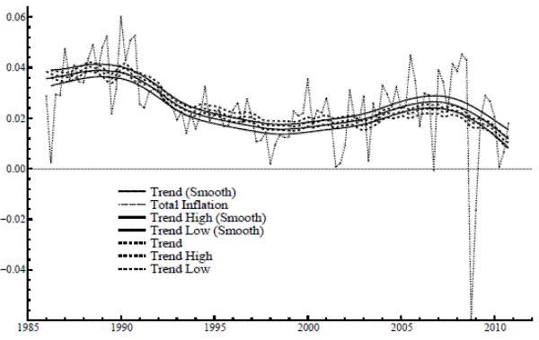Inflation is defined as $4\cdot \log (P_{t}/P_{t-1})$ for price index $% P_{t}$ . Inflation fluctuations appear to have a different structure prior to the sample used here; for example, as apparent in Figure 1, there is no episode, post-mid 80s, comparable to the Great Inflation of the 70s and early 80s. Following this time of high levels and volatile movements, inflation seems to have settled into a different pattern of variation, with a more stable level and with temporary components tending to dissipate rapidly. Economists have discussed various reasons for this new regime, such as a more effective anchoring of inflation expectations.

We estimate the models by Maximum Likelihood³. Though the computation of the likelihood relies on Gaussian distributions, the assumption of normality is actually not needed for the efficiency of the resulting MLEs; see Taniguchi and Kakizawa (2000). With the model cast in state space, the likelihood is evaluated for each set of parameter values using the prediction error decomposition from the Kalman filter; see Harvey (1989) or Durbin and Koopman (2001). The parameter estimates are computed by optimizing over the likelihood surface. Programs were written in the Ox language (Doornik, 1998) and included the Ssfpack library of state space functions (Koopman et. al., 1999) for parameter estimation routines.

Local level results are in Table 1 for the univariate case. While the value of $\sigma _{\eta }^{2}$ has a similar magnitude for core and total, the variance of the irregular is far larger for total inflation. The application of the signal extraction formulas, given the estimated parameters, yields the trends shown in Figure 1. The confidence bands around the trends represent one standard deviation above and below the conditional expectation - the point estimate - taken at all time periods. Each trend meanders throughout the sample, its basic level evolving slowly over the sample period, and it also undergoes frequent and subtle adjustments on a quarterly basis (due to scaling, this is more evident in the graph for core). Such an adaptive level seems reasonable to the extent that underlying inflation is affected by factors that are constantly changing. The signal-noise ratio $q=\sigma _{\eta }^{2}/\sigma _{\epsilon }^{2}$ indicates the relative variability of trend and noise (for a given model structure). The value of reported in the table is much greater for core; this contrast gives a precise statistical depiction and quantifies the informal expression that "core inflation has more signal".

Table 1 also reports three measures of performance and diagnostics. Analogous to the usual regression fit, $R_{D}^{2}$ is the coefficient of determination with respect to first differences; the values in the table indicate that a sizeable fraction of overall variation is explained by the models beyond a random walk, especially for total, where the extraction of the more volatile irregular in producing the trend leads to a favorable fit. The Box-Ljung statistic is based on the first residual autocorrelations; here . The degrees of freedom for the chi-squared distribution of is , where is the number of model parameters, so the 5% critical value for $\chi ^{2}(9)$ is about 16.9. Core and total inflation have roughly equivalent values of clearly below the 5% cutoff. The trade-off between fit and parsimony is expressed in the Akaike Information Criterion (AIC), defined by $AIC\ =-2\log \hat{L}% +2k,$ where $\log \hat{L}$ is the maximized log-likelihood - see (12).

The set of results for the bivariate case, shown in Table 2, confirm the utility of including the core inflation series in the model. Relative to univariate, the statistic for total declines modestly for the bivariate model, while the coefficient of determination rises significantly, with $% R_{D}^{2}$ now measuring over 35% for total inflation. Shared parameters are shown in Table 2b; the close connection between the two series mainly appears in the trends, for which the correlation between the disturbances is estimated as unity. The cross-correlation for the irregulars takes on a smaller positive value of about $\nu _{\epsilon }=0.5$ . As the perfect correlation condition holds, we may directly reformulate the model as having a single common trend. As reported in Table 2b, $\theta$ is somewhat less than one; the AIC decrease reflects the reduction in the number of parameters (values of AIC can be used to compare common and related trends models for either the LLM or STM, but cannot be used to compare an LLM to an STM, because they have different orders of integration.) Figure 2 shows the resulting trend in total inflation and compares it with the univariate output. The solid lines pertain to the bivariate estimates. There are noticeable differences in both the trajectory of the bivariate trend and in the substantially reduced degree of uncertainty associated with its estimation.

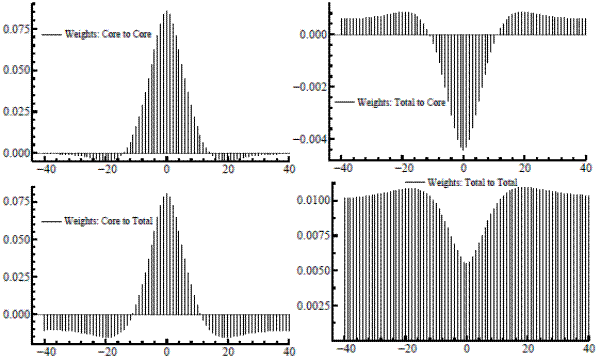
We can now use our signal extraction results to show how the model-based estimator makes optimal use of the information that core inflation gives about the trend in total. The filters, estimated from the model and applied to bivariate dataset, have coefficients in the form of $2\times 2$ weight matrices. An equivalent formulation expresses the bivariate filter as a $2\times 2$ matrix of scalar filters of the usual form; for each element, figure 3 plots each filter weight against the time separation between weighted observation and signal location. The core-to-core weighting pattern in the upper-left box nearly matches the decay pattern of an exponential on each side (there is a slight discrepancy as the weights dip just below zero at the ends). Apart from a very slight constant offset, the weights for total-to-core seem to follow a negative double exponential. Therefore, the current and adjacent values of core inflation are somewhat overweighted, with a modestly-valued moving average of total inflation subtracted. (The small constant offset is due simply to the linear relationship between the two trends.) The bottom-left box shows the core-to-total weights, also resembles a shifted double exponential (with a slightly reduced maximum, compared to core-to-core, to dampen the trend variability a bit). A negative offset is now readily apparent, with the weights going negative after five lags or so, again, from the linear linkage. This kernel is then set against a total-to-total pattern which, like the total-to-core cross filter, has the shape of an inverted double exponential, adjusted by a fixed amount.

The gain functions (for the hypothetical, doubly infinite series) are shown in figure 4. The filter for core-to-core has the usual shape of a low-pass filter, representing a standard focus on low frequencies. The gradual decay of the core-to-core low-pass results from the slow decline of the trend pseudo-spectrum and its overlap with the flat spectrum of the white noise irregular. The gain rises modestly above unity at the low end, indicating a small expansion of amplitudes. Correspondingly, the cross-gain for total-to-core is less than or equal to zero everywhere, reflecting an opposite effect due to total inflation.

As the major portion of the trend in total is assessed by smoothing the core rate, this leads to a core-to-total filter that also resembles a low-pass filter. Now the gain reaches a maximum somewhat below unity, so the filter diminishes slightly the strength of the trend core movements; this contribution is then combined with another reflected (about the frequency-axis) low-pass filter applied to total.

For the smooth trend model, given in (15), the direction adjusts gradually, suggesting slowly changing long-run factors. While the smooth trend model has been successfully applied in research such as Harvey and Trimbur (2003), who examine cycles and trends in economic activity series, the multivariate smooth trends model has not yet been used for inflation data. Now, the specification allows trend inflation to increase or decrease going forward, with the rate of change subject to permanent shocks, whereas the local level model simply projects the current level ahead. As a result, it gives scope for a different view of trend inflation connected to most significant and long-run transitions in the rate over the sample period.

The results, shown in Tables 3 and 4, indicate the smooth trend as another effective tool for inflation, as there is little difference in the fit measure and diagnostics relative to the local level model. There is again a clear improvement in the fit and residual serial correlation in moving to the bivariate model. For the I(2) model, the trends in Figure 5 show stable variation for which the major trending phases and turning points become clearer, than for the more reactive local level. Basically, the estimated trend of the I(2) model concentrates on the lowest frequency, major transitions, for instance, the persistent rise in trend inflation moving into the mid-2000's, followed by stalled gains and a peak during 2007.

The correlation between the slope disturbances is unity, signifying a very close connection. as the pace of adjustment of trend moves together for core and total. Figure 6 contrasts the resulting trend with the univariate output. The solid lines, which show the estimates and confidence bands, indicate that the path of the bivariate trend exhibits somewhat more variation over the sample and is estimated with greater precision. The associated common trend model has the form of (16) with the loading on core normalized to one and a load parameter $\theta$ applied to total. The reported value of $\theta$ is close to one. The weighting kernels for this case are shown in Figure 7. Compared to the local level case, the trend weights for core-to-core are spread over a longer range, with a slower rate of decay with lag length. This difference in weighting pattern gives rise to the smoother trend. As before, a weighted average (offset) of the total inflation series is subtracted from smoothed core inflation (also offset) to form the trend estimate in each series.

From the frequency domain perspective, the persistence in the direction of the trend and its relative smoothness result from greater concentration on low frequencies than for the random walk trend. The resulting set of low-pass filters for the smooth trend model is shown in figure 8. For both series, the gain applied to core inflation cuts off more sharply than the gains in figure 4, and this contribution is set against a negative gain, operating on total inflation, that also falls to near zero more rapidly. The greater effectiveness of the gain in cutting out high frequencies leads to the contrast in visual properties of the smooth trend compared to the local level case, as indicated in figure 9.

The formulas presented above reveal analytically how to make the most efficient use of series with high relative signal content, whose components correlate with the target's. The substantially higher signal-noise ratio of core, and to some extent also the positive irregular correlation, affects the filter design. A pronounced focus on core, which is actually over-weighted and compensated for by subtracting some signal in total, appears to help avoid large errors in favor of more frequent smaller errors in the signal extraction (as the estimator satisfies the minimum MSE optimality criterion).

Compared to a simple reliance on core, the optimal measurement of trend has some basic differences. In both the local level and smooth trend cases, the estimation of each trend starts with the extraction of noise from core. To extract the trend in total inflation, although the emphasis remains on core, a different moving average is applied to the core rate (adjusted by a linear function compared to the weights for computing core trend), which is then set against a modest weighted average of the total rate. So, the measurement of total's trend relies also to some extent on total (and likewise for the trend in core). Our example with trend inflation illustrates how the possibility of contrasting trend structures, different properties of individual series, and linkages across series, together exert important effects on the weight and gain patterns for signal estimation.

While our illustrations have used simple stochastic trend plus noise models, they already show that the exact optimal weighting of just two series has non-obvious aspects such as a slight over-emphasis on the signalling series compensated by subtracting a weighted average of the noisier target. When using more complex specifications to generate even more refined trend estimates, while the set of determinants would expand to include, for instance, variance-ratios involving disturbances for other components such as cycles, one would encounter the same essential issues as in our illustration. The precise way to best combine two or more series with variable signal content, that may have multiple components, depends now on the matrix structures expressing the complete set of dynamic relationships. Our new results allow us to solve the general formulation of such problems explicitly, that would either lie outside our ability to intuit the optimal extraction of the signal or where reliance on intuition alone would lead to inefficient use of the available data (and would preclude knowledge of the probable error or of the uncertainty in our estimates).

5 Conclusions

Applications of signal extraction intertwines with areas like current analysis, policy-making, and forecasting; in this context, multivariate frameworks may yield more informed and accurate estimates of components of interest, while incorporating more of the available information in the form of additional series and their cross-relationships. Often the economic data involved show nonstationary behavior, and the related stochastic trends across series represent a primary signal of interest, whose estimation also substantially influences the measurement of any other components present in the series.

Here, we have generalized the well-known Wiener-Kolmogorov formula to the situation of interest in econometrics, which represents a key theoretical foundation and allows us to derive new results on signal estimation for multiple economic time series. The effective modelling of co-movements across related time series has been the subject matter of some of the major ongoing developments in econometrics in statistics, and correspondingly, a wide range of multivariate signal extraction systems appear in economics and other fields. The contributions of this paper substantially extend our understanding of such problems; now we can examine the analytical expressions for the optimal set of weight polynomials, applied to the observation vectors, based on the matrix ACGFs or pseudo-ACGFs. The bi-infinite analysis shows, in compact form, precisely how to best use the new information, in addition to the component relationships in the signal's own reference series, to construct estimates. When series with high signal content are readily available, as in the total-core inflation example, we can derive the adjustment and shifting of model-based weightings on the observations, quantifying how it depends on the cross-correlations and variances. This mathematical precision, together with the accompanying insight and knowledge about the signal estimation, may provide the basis for improved treatment of and better understanding of existing contexts. Our formulas also allow us to derive new signal estimators for multiple nonstationary time series, expanding the scope of methodology in economics and other fields.

The finite sample time-domain formulas, which we have used for the actual application of the filters, account for the dependence of the correct optimal filters on series length and signal location. The new theoretical content consists of general analytical expressions for weight patterns, that reveal precisely how series length, signal location, and parameters (including those governing dynamic linkages among series) jointly affect the estimators. From a methodological perspective, our contribution expands the array of available computational strategies, in particular the widely used state space approach. The direct matrix approach includes extensions, such as long-memory, not easily handled in state space. As another example, it allows us to explore signal extraction theory in the presence of time variation in variances - a model aspect of extensive interest in the time series literature - in the multivariate extension to McElroy (2008), who showed initial results for the univariate case.

While our results cover ground complementary to the state space approach, our method offers a different, direct route to calculation (results in Bell and Hillmer (1991) indicate that a correctly initialized Kalman filter will produce Gaussian conditional expectations that are in agreement with standard initial values assumptions such as those made in this paper). The complete functional form of the optimal asymmetric filters for multiple series may also prove useful toward improving practice, as, for instance, signal detection properties toward the end of the available data remain of considerable importance for researchers and, perhaps, policymakers. The method can also readily produce useful additional information, e.g., quantities like signal velocity, or rates of change. As another example, we may examine signal estimation diagnostics that indicate performance in this context, analogous to statistical measures for specification tenability in a model comparison context.

In addition to providing the base for eliciting movements of interest (or certain properties of these movements), signal-noise structures also represent candidate classes of time series models, useful for the typical problems like historical summary and interpretation and explanatory analysis as well as forecasting. These formulations offer useful windows into patterns in fluctuations, and we can handle co-integration with common driving forces for the stochastic trends or analogously, linked stationary, serially correlated elements in groups of series. So we can unify modelling, descriptive analysis, and forecasting with signal extraction frameworks, including classic ones - connected to the kind of macroeconomic story-telling useful for discussions among economists and policy-makers - like those used to estimate trends (such as potential output or the NAIRU) or business cycle components.

Based on the core property of optimality and adaptability to time series dynamics, our contributions provide a cornerstone for signal extraction theory and estimator design in econometrics: completing a well-known line of contributions (Wiener (1949), Whittle (1963), and Bell (1984)) and generalizing the matrix method, a direct alternative to the popular state space approach with new theoretical content for finite samples. As the formulations we consider include highly general multivariate specifications for nonstationary sets of time series, our results have a broad scope and allow for comprehensive development and investigation of a very wide range of situations, including advances in existing areas like trend analysis, as well as new signal extraction architectures that may emerge from future research and experience with economic fluctuations.

A. Proof of Theorem 1

. The action of each filter on a time series is obtained by replacing by and $\overline{z}$ by $L^{-1}$ . The error process is defined via ${\bf\epsilon}_t = \boldsymbol{W} (L) {\bf y}_t - {\bf s}_t$ . (It is also easy to derive an expression for $1_N - \boldsymbol{W} (z)$ , which has the same formula as (6) but with signal and noise swapped.) Then applying (6) to this error decomposition yields

$\displaystyle {\bf\epsilon}_t$	$\displaystyle = \widetilde{\bf\Gamma}_{\bf w}^{-1} (L) \left( \widetilde{\bf\Gamma}_{{\bf v}, {\bf w}} (L) {\bf\Gamma}_{{\bf u}, {\bf w}} (L) - \widetilde{\bf\Gamma}_{{\bf u}, {\bf w}} (L) {\bf\Gamma}_{{\bf v}, {\bf w}} (L) \right) {\bf\Gamma}_{\bf w}^{-1} (L) {\bf w}_t$
	$\displaystyle + \widetilde{\bf\Gamma}_{\bf w}^{-1} (L) \widetilde{\bf\Gamma}_{{\bf u}, {\bf w}} (L) {\bf v}_t - \widetilde{\bf\Gamma}_{\bf w}^{-1} (L) \widetilde{\bf\Gamma}_{{\bf v}, {\bf w}} (L) {\bf u}_t.$

One can swiftly see the stationarity of the error process, as well as its orthogonality to ${\bf w}_{t+h}$ for all

and any

. In the expectation calculations, we can use the Cramer representation for $\{ {\bf w}_t \}$ to get expressions involving integrals - then the fact that the frf is not defined on a set of measure zero becomes irrelevant. Moreover, since the error process only depends on $\{ {\bf u}_t \}$ and $\{ {\bf v}_t \}$ , it is orthogonal to the initial values of the data process as well, by Assumption $M_{\infty }$ . Hence the error process is uncorrelated with $\{ {\bf y}_t \}$ , proving the optimality of the signal extraction filter. The formula for the error spectral density also follows from the above description of the error process.

Under the assumption that the differencing operators are uniform, we have (since diagonal matrices commute with any other matrix)

$\displaystyle \widetilde{\bf\Gamma}_{{\bf v}, {\bf w}} (z) {\bf\Gamma}_{{\bf u}, {\bf w}} (z) \widetilde{\bf\delta} (z)$	$\displaystyle = \widetilde{\bf\Gamma}_{\partial {\bf v}} (z) {\bf\Gamma}_{\partial {\bf u}} (z)$
$\displaystyle \widetilde{\bf\Gamma}_{{\bf u}, {\bf w}} (z) {\bf\Gamma}_{{\bf v}, {\bf w}} (z) \widetilde{\bf\delta} (z)$	$\displaystyle = \widetilde{\bf\Gamma}_{\partial {\bf u}} (z) {\bf\Gamma}_{\partial {\bf v}} (z).$

Using this relation produces

$\displaystyle \boldsymbol{W} (z)$	$\displaystyle = \widetilde{\bf\Gamma}_{\bf w}^{-1} (z) \left[ \widetilde{\bf\Gamma}_{\partial {\bf u}} (z) + \left( \widetilde{\bf\Gamma}_{\partial {\bf v}} (z) {\bf\Gamma}_{\partial {\bf u}} (z) - \widetilde{\bf \Gamma}_{\partial {\bf u}} (z) {\bf\Gamma}_{\partial {\bf v}} (z) \right) {\bf\Gamma}_{\bf w}^{-1} (z) \right]$
	$\displaystyle = \widetilde{\bf\Gamma}_{\bf w}^{-1} (z) \left[ \widetilde{\bf\Gamma}_{\partial {\bf u}} (z) {\bf\Gamma}_{\partial {\bf u}} (z) + \widetilde{\bf\Gamma}_{\partial {\bf v}} (z) {\bf\Gamma}_{\partial {\bf u}} (z) \right] {\bf\Gamma}_{\bf w}^{-1} (z)$
	$\displaystyle = {\bf\Gamma}_{\partial {\bf u}} (z) {\bf\Gamma}_{\bf w}^{-1} (z).$

Similar substitutions in the error spectral density produce, after much algebra, the stated formula. $\quad \Box$

B. Proof of Proposition 1.

The spectral density of the differenced data process is

$\displaystyle \boldsymbol{F}_{\bf w} (\lambda) = {\vert\delta_{\bf n} (z) \vert}^2 \Xi (z) \Sigma_{\bf\zeta} \Xi^{\prime} (\overline{z}) + {\vert\delta_{\bf s} (z) \vert}^2 \Omega (z) \Sigma_{\bf\kappa} \Omega^{\prime} (\overline{z}).$

For any fixed $\lambda$ , this expression is the linear combination of a positive definite and a non-negative definite matrix. So long as ${\vert\delta_{\bf s} (z) \vert}^2$ is nonzero, $\boldsymbol{F}_{\bf w} (\lambda)$ will be invertible, but otherwise the matrix is singular. Let $p(\lambda) = {\vert\delta_{\bf n} (z) \vert}^2$ and $q(\lambda) = {\vert\delta_{\bf s} (z) \vert}^2$ for short. If $\lambda_s$ is a root of

, then

$\displaystyle {\bf F}_{\bf w} (\lambda_s) = p (\lambda_s) \Xi (z_s) \Sigma_{\bf\zeta} \Xi^{\prime} (\overline{z_s}),$

where $z_s = e^{-i \lambda_s }$ . If this matrix has determinant zero, then either $\vert \Sigma_{\bf\zeta}\vert = 0$ or there exists some matrix

(depending on $\lambda_s$ ) such that $a^{\prime} \Xi (z_s) = 0$ . The former case corresponds to co-linearity of the signal core process, whereas the latter case is discussed further below. If the signal core process is co-linear, then from the singular value decomposition of $\Sigma_{\bf \zeta}$ we can write this matrix as $\Theta \Sigma_{\bf\eta} \Theta^{\prime}$ . Here $\Sigma_{\bf\eta}$ has reduced dimension corresponding to the number of nonzero eigenvalues of $\Sigma_{\bf \zeta}$ , and $\Theta$ is rectangular. Then the Sherman-Morrison-Woodbury formula (Golub and Van Loan, 1996) yields

$\displaystyle \boldsymbol{F}_{\bf w}^{-1} (\lambda )$	$\displaystyle = q^{-1} (\lambda) { \left[ \Omega (z) \Sigma_{\bf\kappa} \Omega^{\prime} (\overline{z}) \right] }^{-1} - \frac{ p (\lambda) }{ q (\lambda) } { \left[ \Omega (z) \Sigma_{\bf\kappa} \Omega^{\prime} (\overline{z}) \right] }^{-1} \Xi (z) \Theta \Sigma_{\bf\eta}$
	$\displaystyle \cdot { \left\{ q (\lambda) 1_N + p(\lambda) \Theta^{\prime} \Xi^{\prime} (\overline{z}) { \left[ \Omega (z) \Sigma_{\bf\kappa} \Omega^{\prime} (\overline{z}) \right] }^{-1} \Xi (z) \Theta \Sigma_{\bf\eta} \right\} }^{-1}$
	$\displaystyle \cdot \Theta^{\prime} \Xi^{\prime} (\overline{z}) { \left[ \Omega (z) \Sigma_{\bf\kappa} \Omega^{\prime} (\overline{z}) \right] }^{-1}.$

This formula is quite informative: the above derivation shows that $q \boldsymbol{F}_{\bf w}^{-1}$ is bounded for all $\lambda$ , even in a neighborhood of $\lambda_s$ . Unfortunately, the matrix $\boldsymbol{F}_{\bf w}$ is not invertible at $\lambda_s$ , and the rate of explosion of $q^{-1} (\lambda)$ is generally such that the Whittle likelihood (see (3.1.5 of Taniguchi and Kakizawa (2000)) is not well-defined.

However, the frf (7) for any $\lambda$ such that $q(\lambda) \neq 0$ is given by

$\displaystyle \boldsymbol{W} (z)$	$\displaystyle = 1_N - q(\lambda) \Omega (z) \Sigma_{\bf\kappa} \Omega^{\prime} (\overline{z}) \boldsymbol{F}_{\bf w}^{-1} (\lambda)$
	$\displaystyle = p (\lambda) \Xi (z) \Theta \Sigma_{\bf\eta} \cdot { \left\{ q (\lambda) 1_N + p(\lambda) \Theta^{\prime} \Xi^{\prime} (\overline{z}) { \left[ \Omega (z) \Sigma_{\bf\kappa} \Omega^{\prime} (\overline{z}) \right] }^{-1} \Xi (z) \Theta \Sigma_{\bf\eta} \right\} }^{-1}$
	$\displaystyle \cdot \Theta^{\prime} \Xi^{\prime} (\overline{z}) { \left[ \Omega (z) \Sigma_{\bf\kappa} \Omega^{\prime} (\overline{z}) \right] }^{-1},$

and the limit as $\lambda$ tends $\lambda_s$ of this is well-defined; we set $q (\lambda) = 0$ and $p(\lambda) = p(\lambda_s)$ (which is nonzero, since the signal and noise differencing polynomials are relatively prime by assumption). That is,

$\displaystyle \boldsymbol{W} (z_s)$	$\displaystyle = p (\lambda_s) \Xi (z_s) \Theta \Sigma_{\bf\eta} \cdot { \left\{ p(\lambda_s) \Theta^{\prime} \Xi^{\prime} (\overline{z_s}) { \left[ \Omega (z_s) \Sigma_{\bf\kappa} \Omega^{\prime} (\overline{z_s}) \right] }^{-1} \Xi (z_s) \Theta \Sigma_{\bf\eta} \right\} }^{-1}$
	$\displaystyle \cdot \Theta^{\prime} \Xi^{\prime} (\overline{z_s}) { \left[ \Omega (z_s) \Sigma_{\bf\kappa} \Omega^{\prime} (\overline{z_s}) \right] }^{-1}.$	(A.1)

Now let us treat the case that the innovations are not co-linear, and yet $a^{\prime} \Xi (z) = 0$ at some measure zero set of frequencies (with a different

for each frequency $\lambda$ ). Let $\Lambda$ denote the set of frequencies where ${\bf F}_{\bf w}$ is invertible, so that

$\displaystyle {\bf\Gamma}_{\partial {\bf u} } (z ) {\bf\Gamma}_{\bf w}^{-1} (z) = 1_N - q(\lambda) { \left( 1_N + p (\lambda) {\bf F}_{\bf u} (\lambda) {\bf F}_{\bf v}^{-1} (\lambda) \right) }^{-1},$

which is well-defined for all frequencies $\lambda$ ; for $\lambda \not\in \Lambda$ , we can take the limit as $\lambda$ tends $\lambda_s$ , since the matrix inverse in the above expression always exists. The limit is just

, so ${\bf W} (z)$ can be continuously extended to all frequencies. This completes the proof. $\quad \Box$

C. Proof of Theorem 2.

The invertibility of each $M^{jj}$ follows from the univariate argument in McElroy (2008), using the fact that $\delta _{\mathbf{s}}^{(j)}$ and $\delta _{\mathbf{n}}^{(j)}$ share no common factors. The signal error for the th signal is

$\displaystyle \epsilon^{(j)} = \widehat{\mathbf{s}}^{(j)} - \mathbf{s}^{(j)} = \sum_{k \neq j} F^{jk} {\mathbf{y}}^{(k)} + F^{jj} {\mathbf{n}}^{(j)} - (1 - F^{jj}) \mathbf{s}^{(j)}.$

Optimality of the matrix formulas follows from demonstrating that $\epsilon^{(j)}$ is orthogonal to ${\mathbf{y}}$ , the stacking of the individual data vectors ${\mathbf{y}}^{(k)}$ . As in Bell (1984), we can write ${\mathbf{y}}$ as a linear combination of ${\mathbf{w}}$ and various initial values for all the component series. Utilizing Assumption

, it is then sufficient to demonstrate that $\epsilon^{(j)}$ is uncorrelated with ${\mathbf{w}}$ . Noting the formula for $1 - F^{jj}$ , we obtain

$\displaystyle \epsilon^{(j)}$	$\displaystyle = \sum_{k \neq j} {M^{jj}}^{-1} \sum_{\ell =1}^N \left( C^{j \ell} - D^{j \ell} \right) \Gamma_{\mathbf{w}}^{\ell k} {\mathbf{w}}^{(k)}$
	$\displaystyle + { M^{jj} }^{-1} \left[ {\Delta_{\mathbf{n}}^{(j)} }^{\prime} {\Sigma_{\mathbf{v}}^{jj}}^{-1} {\mathbf{v}}^{(j)} + \Sigma_{\ell \neq j} \left( C^{j \ell} - D^{j \ell} \right) \Gamma_{\mathbf{w}}^{\ell j} \underline{\Delta}_{\mathbf{s}}^{(j)} {\mathbf{v}}^{(j)} \right]$
	$\displaystyle - { M^{jj} }^{-1} \left[ {\Delta_{\mathbf{s}}^{(j)} }^{\prime} {\Sigma_{\mathbf{u}}^{jj}}^{-1} {\mathbf{u}}^{(j)} + \Sigma_{\ell \neq j} \left( C^{j \ell} - D^{j \ell} \right) \Gamma_{\mathbf{w}}^{\ell j} \underline{\Delta}_{\mathbf{n}}^{(j)} {\mathbf{u}}^{(j)} \right].$

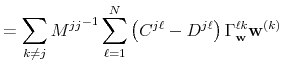Next, we show that the covariance between this error vector and each ${\mathbf{w}}^{(p)}$ is zero for each

. Noting (11), we obtain

$\displaystyle [ \mathbb{E} \epsilon^{(j)} {{\mathbf{w}}^{(p)}}^{\prime} ]$	$\displaystyle = \sum_{k \neq j} {M^{jj}}^{-1} \sum_{\ell =1}^N \left( C^{j \ell} - D^{j \ell} \right) \Gamma_{\mathbf{w}}^{\ell k} \Sigma_{\mathbf{w}}^{kp}$
	$\displaystyle + { M^{jj} }^{-1} \left[ {\Delta_{\mathbf{n}}^{(j)} }^{\prime} {\Sigma_{\mathbf{v}}^{jj}}^{-1} \Sigma_{\mathbf{v}}^{jp} {\underline{\Delta}_{\mathbf{s}}^{(p)}}^{\prime} + \Sigma_{\ell \neq j} \left( C^{j \ell} - D^{j \ell} \right) \Gamma_{\mathbf{w}}^{\ell j} \underline{\Delta}_{\mathbf{s}}^{(j)} \Sigma_{\mathbf{v}}^{jp} {\underline{\Delta}_{\mathbf{s}}^{(p)}}^{\prime} \right]$
	$\displaystyle - { M^{jj} }^{-1} \left[ {\Delta_{\mathbf{s}}^{(j)} }^{\prime} {\Sigma_{\mathbf{u}}^{jj}}^{-1} \Sigma_{\mathbf{u}}^{jp} {\underline{\Delta}_{\mathbf{n}}^{(p)}}^{\prime} + \Sigma_{\ell \neq j} \left( C^{j \ell} - D^{j \ell} \right) \Gamma_{\mathbf{w}}^{\ell j} \underline{\Delta}_{\mathbf{n}}^{(j)} \Sigma_{\mathbf{u}}^{jp} {\underline{\Delta}_{\mathbf{n}}^{(p)}}^{\prime} \right]$
	$\displaystyle = {M^{jj}}^{-1} \sum_{\ell=1}^N \left( C^{j \ell} - D^{j \ell} \right) \sum_{k \neq j} \Gamma_{\mathbf{w}}^{\ell k} \Sigma_{\mathbf{w}}^{kp}$
	$\displaystyle + { M^{jj} }^{-1} \Sigma_{\ell \neq j} \left( C^{j \ell} - D^{j \ell} \right) \Gamma_{\mathbf{w}}^{\ell j} \Sigma_{\mathbf{w}}^{jp}$
	$\displaystyle + { M^{jj} }^{-1} \left( C^{jp} - D^{jp} \right).$

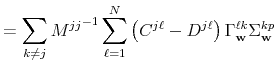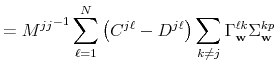Consider the first term. By the definition of $\Gamma_{\mathbf{w}}^{\ell k}$ , we know that $\sum_k \Gamma_{\mathbf{w}}^{\ell k} \Sigma_{\mathbf{w}}^{kp}$ is a matrix of zeroes unless $\ell = p$ , in which case it is an identity matrix. As a result, the first term can be rewritten as

$\displaystyle {M^{jj}}^{-1} \left( C^{jp} - D^{jp} \right) - {M^{jj}}^{-1} \sum_{\ell =1}^N \left( C^{j \ell} - D^{j \ell} \right) \Gamma_{\mathbf{w}}^{\ell j} \Sigma_{\mathbf{w}}^{jp}.$

The left-hand term here cancels with the third term above. The right-hand term here actually cancels with the second term above, since when $\ell=j$ we get

$\displaystyle {\Delta_{\mathbf{s}}^{(j)} }^{\prime} {\Sigma_{\mathbf{u}}^{jj}}^{-1} \Sigma_{\mathbf{u}}^{jj} { \underline{\Delta}_{\mathbf{n}}^{(j)} }^{\prime} - \Delta_{\mathbf{n}}^{(j)} {\Sigma_{\mathbf{v}}^{jj} }^{-1} \Sigma_{\mathbf{v}}^{jj} {\underline{\Delta}_{\mathbf{s}}^{(j)} }^{\prime} = \Delta^{(j)} - \Delta^{(j)} = 0$

by (10). This completes the proof of optimality. The signal extraction covariance matrix is produced by using the above expression for $\epsilon^{(j)}$ in $\mathbb{B}[ \epsilon^{(j)} {\epsilon^{(k)}}^{\prime}]$ , after much algebra.

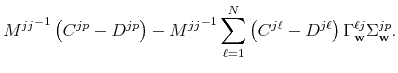
To prove the matrix form of the results, note that the th block matrix of the putative formula for is

	$\displaystyle \sum_{\ell=1}^N {M^{j \ell} }^{-1} \left( \widetilde{B}^{\ell k} + \sum_{p,q=1}^N \left( C^{\ell p} - D^{\ell p} \right) \Gamma_{\mathbf{w}}^{pq} \Delta^{qk} \right)$
	$\displaystyle = {M^{jj} }^{-1} \left( B^{jk} + \sum_{p=1}^N \left( C^{jp} - D^{jp} \right) \Gamma_{\mathbf{w}}^{pk} \Delta^{(k)} \right),$

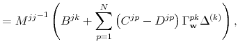using the block-diagonal structure of

, $\widetilde{B}$ , and $\Delta$ . The formula for $F^{jk}$ can now be recognized by the above expression. Similar calculations establish the formulas for $F^{jj}$ and

. $\quad \Box$

Acknowledgements Thanks to participants at the NBER/NSF time series conference, held at Michigan State University in September 2011, as well as those who attended the College Park seminar in October 2011 and the FRB seminar in November 2011. Thanks in particular to William Bell, Scott Holan, Ben Kedem, Seth Pruitt, Elmar Mertens, Barbara Rossi, Jeremy Rudd, Aaron Smith and Marc Wildi for helpful discussion.

Bibliography

Ansley C. and Kohn, R., (1985)

Estimation, filtering, and smoothing in state space models with incompletely specified initial conditions. Ann. Statist. 13, 1286-1316.

Azevedo J. Koopman, S., and A. Rua, (2006)

Tracking the Business Cycle of the Euro Area: A Multivariate Model-Based Bandpass Filter. Journal of Business and Economic Statistics 24, 278-90.

Basistha A. and Startz, D., (2008)

Measuring the NAIRU with reduced uncertainty: a multiple-indicator common-cycle approach. Review of Economics and Statistics 90, 805-811.

Bell, W., (1984)

Signal extraction for nonstationary time series. The Annals of Statistics 12, 646-664.

Bell W., (2004)

On RegComponent time series models and their applications. In A.C. Harvey, S.J. Koopman, and N. Shephard (Eds.), State Space and Unobserved Component Models: Theory and Applications. Cambridge, UK: Cambridge University Press.

Bell W. and Hillmer, S., (1991)

Initializing the Kalman filter for nonstationary time series models. Journal of Time Series Analysis 12, 283-300.

Brockwell, P. and Davis, R., (1991)

Time Series: Theory and Methods, 2nd Ed. New York: Springer.

Cogley T., (2002)

A simple adaptive measure of core inflation. Journal of Money, Credit and Banking 34, 94-113.

Cogley T. and A. Sbordone, (2008)

Trend inflation, indexation, and inflation persistence in the new Keynesian Phillips curve. American Economic Review 98, 2101-2126.

Doornik J., (1998)

Object-oriented Matrix Programming using Ox 2.0. London: Timberlake Consultants Press.

Durbin J. and Koopman, S., (2001)

Time Series Analysis by State Space Methods. Oxford University Press.

Engle R. and Granger, C., (1987)

Cointegration and error correction: representation, estimation, and testing. Econometrica 55, 251-276.

Golub, G. and Van Loan, C., (1996)

Matrix Computations. Baltimore and London: The Johns Hopkins University Press.

Gómez V., (2006)

Wiener-Kolmogorov filtering and smoothing for multivariate series with state-space structure. Journal of Time Series Analysis 28, 361-385.

Harvey A., (1989)

Forecasting, Structural Time Series Models and the Kalman Filter. Cambridge, Cambridge University Press.

Harvey A. C., and Trimbur T., (2003)

General model-based filters for extracting cycles and trends in economic time series. Review of Economics and Statistics 85, 244-255.

Johansen S., (1988)

Statistical analysis of cointegration vectors. Journal of Economic Dynamics and Control 12, 231-254.

Kiley Michael T., (2008)

Estimating the Common Trend Rate of Inflation for Consumer Prices and Consumer Prices Excluding Food and Energy Prices, Finance and Economics Discussion Series 2008-38. Board of Governors of the Federal Reserve System..

Koopman S. J. and Harvey, A. C., (2003)

Computing observation weights for signal extraction and filtering. Journal of Economic Dynamics and Control 27, 1317-33.

Koopman S., Shephard, N., and Doornik, J., (1999)

Statistical algorithms for models in state space using SsfPack 2.2. Econometrics Journal 2, 113-166.

Lütkepohl H., (2006)

New Introduction to Multiple Time Series Analysis. Springer-Verlag, Berlin.

McElroy T. and Sutcliffe, A., (2006)

An iterated parametric approach to nonstationary signal extraction. Computational Statistics and Data Analysis, Special Issue on Signal Extraction 50, 2206-2231.

McElroy T., (2008)

Matrix formulas for nonstationary ARIMA signal extraction. Econometric Theory 24, 1-22.

Nyblom J. and Harvey, A., (2000)

Tests of common stochastic trends. Econometric Theory 16, 176-199.

Stock J. and Watson, M., (1988)

Testing for common trends. Journal of the American Statistical Association 83, 1097-1107.

Stock J. and Watson, M., (2007)

Why Has U.S. Inflation Become Harder to Forecast? Journal of Money, Credit and Banking S39, 3-33.

Taniguchi M. and Kakizawa, Y., (2000)

Asymptotic Theory of Statistical Inference for Time Series. Springer-Verlag, New York.

Trimbur T. M., (2010)

Stochastic level shifts and outliers and the dynamics of oil price movements. International Journal of Forecasting 26, 162-179.

Whittle P., (1963)

Prediction and Regulation. London: English Universities Press.

Wiener N., (1949)

The Extrapolation, Interpolation, and Smoothing of Stationary Time Series with Engineering Applications. New York: Wiley.

Table 1: Parameter estimates, Univariate Local Level Models

	$\sigma _{\eta }^{2}$	$\sigma _{\epsilon }^{2}$		$% R_{D}^{2}$
Core	5.82e-006	1.77e-005	0.329	0.164	13.42	-750.96
Total	7.41e-006	0.000172	0.0431	0.261	13.26	-559.01

Results for sample period 1986Q1 to 2010Q4 for models of the form (13) with ${\small N=1}$ . The parameter $% {\small\sigma }_{\eta }^{2}$ corresponds to the variance of the trend disturbance, in this case a level disturbance, and ${\small\sigma }% _{\varepsilon }^{2}$ is the irregular variance; ${\small q=\sigma }% _{{\small\eta }}^{{\small 2}}/{\small\sigma }_{{\small\varepsilon }}^{% {\small 2}}$ is the signal-noise ratio . ${\small R}_{{\small D}% }^{{\small 2}}$ is the coefficient of determination with respect to first differences, and ${\small Q(P)}$ is the Box-Ljung statistic based on the first ${\small P=10}$ residual autocorrelations. $% {\small AIC}$ is the Akaike Information Criterion, given by $% {\small -2}$ log ${\small\widehat{L}+2k},$ where log $% \widehat{{\small L}}$ is the maximized log-likelihood.

Table 2: Parameter estimates, Bivariate Local Level Model

Table 2a: Own Parameter estimates

	$\sigma _{\zeta }^{2}$	$\sigma _{\epsilon }^{2}$		$% R_{D}^{2}$
Core	5.18946e-006	1.84607e-005	0.281	0.179	11.08
Total	3.66532e-006	0.000177859	0.0206	0.3552	12.77

Results for sample period 1986Q1 to 2010Q4 for a model of the form (13) with ${\small N=2}$ . For the series indicated in the left-most column, the parameter ${\small\sigma }_{{\small % \eta }}^{{\small 2}}$ corresponds to the variance of the level disturbance and ${\small\sigma }_{{\small\varepsilon }}^{{\small 2}}$ is the irregular variance; ${\small q=\sigma }_{{\small\eta }}^{% {\small 2}}/{\small\sigma }_{{\small\varepsilon }}^{{\small 2}}$ is the signal-noise ratio . ${\small R}_{{\small D}}^{{\small 2}}$ is the coefficient of determination with respect to first differences, and $% {\small Q(P)}$ is the Box-Ljung statistic based on the first $% {\small P=10}$ residual autocorrelations.

Table 2b: Linked Parameter estimates

$\nu _{\eta }$	$\nu _{\epsilon }$	(Related)	$\theta$	Common)
1.000	0.49832	-1349.25	0.840	-1351.25

Results for sample period 1986Q1 to 2010Q4 for a model of the form (13) with ${\small N=2}$ . The parameter $% {\small\nu }_{{\small\eta }}$ corresponds to the correlation between the level disturbances in the two series, and ${\small\nu }_{% {\small\varepsilon }}$ is the irregular variance. ${\small AIC}$ is given by ${\small -2}$ log ${\small\widehat{L}+2k},$ where log $\widehat{{\small L}}$ where log $\widehat{% {\small L}}$ is the maximized log-likelihood. ${\small AIC}$ (Related) is the Akaike Information Criterion for (13) where ${\small\nu }_{{\small\eta }}$ is an estimated parameter. For the common levels form, (14), $% {\small\theta }$ is the load factor, applied to the trend in core, that gives the trend in total; ${\small AIC}$ (Common) is the Akaike Information Criterion of the model.

Table 3: Parameter estimates, Univariate Smooth Trend Models

	$\sigma _{\zeta }^{2}$	$\sigma _{\epsilon }^{2}$		$% R_{D}^{2}$
Core	6.36e-008	2.33e-005	0.00273	0.133	16.37	-748.82
Total	6.17e-008	0.000185	0.000334	0.22	12.64	-555.06

Results for sample period 1986Q1 to 2010Q4 for models of the form (15) with ${\small N=1}$ . The parameter ${\small % \sigma }_{{\small\zeta }}^{{\small 2}}$ is the slope disturbance variance parameter, and ${\small\sigma }_{{\small\varepsilon }}^{{\small 2}}$ is the irregular variance; ${\small q=\sigma }_{{\small\zeta }% }^{{\small 2}}/{\small\sigma }_{{\small\varepsilon }}^{{\small 2}}$ is the signal-noise ratio . ${\small R}_{{\small D}}^{{\small 2}}$ is the coefficient of determination with respect to first differences, and ${\small Q(P)}$ is the Box-Ljung statistic based on the first ${\small P=10}$ residual autocorrelations. ${\small % AIC}$ is the Akaike Information Criterion, given by ${\small -2}$ log ${\small\widehat{L}+2k},$ where log $\widehat{{\small L}}$ is the maximized log-likelihood.

Table 4: Parameter estimates, Bivariate Smooth Trend Model

Table 4a: Own Parameter estimates

	$\sigma _{\zeta }^{2}$	$\sigma _{\epsilon }^{2}$		$% R_{D}^{2}$
Core	6.11564e-008	2.34043e-005	0.00261	0.1462	15.3
Total	6.89953e-008	0.000179544	0.000384	0.3457	14.07

Results for sample period 1986Q1 to 2010Q4 for a model of the form (15) with ${\small N=2}$ . For the series indicated in the left-most column, the parameter ${\small\sigma }_{{\small % \zeta }}^{{\small 2}}$ corresponds to the variance of the slope disturbance and ${\small\sigma }_{{\small\varepsilon }}^{{\small 2}}$ is the irregular variance; ${\small q=\sigma }_{{\small\zeta }}^{% {\small 2}}/{\small\sigma }_{{\small\varepsilon }}^{{\small 2}}$ is the signal-noise ratio . ${\small R}_{{\small D}}^{{\small 2}}$ is the coefficient of determination with respect to first differences, and $% {\small Q(P)}$ is the Box-Ljung statistic based on the first $% {\small P=10}$ residual autocorrelations.

Table 4b: Linked Parameter estimates

$\nu _{{\small\zeta }}$	$\nu _{\epsilon }$	Related)	$\theta$	(Common)
1.000	0.513972	-1332.06	1.06219	-1334.06

Results for sample period 1986Q1 to 2010Q4 for a model of the form (15) with ${\small N=2}$ . The parameter ${\small % \nu }_{{\small\zeta }}$ corresponds to the correlation between the slope disturbances in the two series, and ${\small\nu }_{{\small % \varepsilon }}$ is the irregular variance. ${\small AIC}$ is given by ${\small -2}$ log ${\small\widehat{L}+2k},$ where log $\widehat{{\small L}}$ where log $\widehat{{\small L}}$ is the maximized log-likelihood. ${\small AIC}$ (Related) is the Akaike Information Criterion for (15) where ${\small\nu }_{{\small\zeta }}$ is an estimated parameter. For the common slopes form, (16), ${\small\theta }$ is the load factor, applied to the trend in core, that gives the trend in total; ${\small AIC}$ (Common) is the Akaike Information Criterion of the model.

Figure 1: Trend estimates, Univariate Local Level Model, for core and total PCE inflation. Sample is 1986Q1 to 2010Q4

Figure 1: Trend estimates, Univariate Local Level Model, for core and total PCE inflation. Four panels. The figure plots the trends in core and total PCE inflation produced using the results from the univariate local level model. The top two panels deal with core inflation, while the bottom two panels deal with total inflation. In all four panels, the X axis displays time, from the first quarter of 1986 to the fourth quarter of 2010. Top-left panel: Y axis displays level of core inflation, ranging from 0.000 to 0.055. Four variables are plotted: core inflation, the trend produced using the parameters from the local level model, the trend high, and the trend low (the high and low represent one standard deviation above and below the conditional expectation - the point estimate - taken at all time periods). The basic trend levels evolve slowly over the sample period, undergoing frequent and subtle adjustments on a quarterly basis. As for the level of core inflation, it bounces around its trend quite a bit; core inflation begins relatively high, around 0.04, in the late 1980s, then gradually declines until it reaches a level of around 0.015 in the late 1990s; it increases briefly in the mid-2000s, then declines throughout 2008, dipping below 0.01 by late 2008; then it rises briefly again, to above 0.02, and then dips below 0.01 again by the fourth quarter of 2010. Bottom-left panel: Shows the same variables as the top-left panel, but with total inflation instead of core inflation. Y axis displays level of total inflation, ranging from -0.0625 to 0.0625. As with core inflation, the basic trend levels evolve slowly over the sample period and undergo frequent and subtle adjustments on a quarterly basis. As for the level of total inflation, it follows a path similar to core inflation, but total inflation shows greater variance, and at one point enters strikingly negative territory, dipping to around -0.06 in late 2008, after which it rises to around 0.025 in 2009 before settling around 0.010 in the fourth quarter of 2010. Top-right panel: Y axis displays the level of the Irregular (εt) for core inflation, ranging from -0.010 to 0.010, with a horizontal line drawn at y = 0. The Irregular for core inflation in the top-right panel reflects the movement of core inflation around its trend in the top-left panel, but the mean of the Irregular is by definition equal to zero. The Irregular seems to bounce above and below zero at random. Bottom-right panel: Y axis displays the level of the Irregular (εt) for total inflation, ranging from -0.075 to 0.025 with a horizontal line drawn at y = 0. The movement of the Irregular for total inflation reflects the movement of total inflation around its trend in the bottom-left panel, but the mean of the Irregular is zero. The variance of the Irregular is apparently larger for total inflation than for core inflation. Because the movement of the Irregular mimics the movement of the total inflation variable in the bottom-left panel, the Irregular also dips into exceptionally negative territory in late 2008.
*Figure 1 can be examined alongside Figure 5, which shows the trends produced using parameters from the Bivariate Smooth Trend Model rather than the Univariate Local Level Model used here.

Figure 2: Trend estimates, Univariate and Bivariate Local Level Model, for total PCE inflation. Sample is 1986Q1 to 2010Q4

Figure 2: Trend estimates, Univariate and Bivariate Local Level Model, for total PCE inflation. One panel. Figure 2 compares the results from the bivariate local level model and the results from the univariate local level model, both with respect to total inflation. X axis shows time, from the first quarter of 1986 to the fourth quarter of 2010; Y axis displays level of total inflation, ranging from -0.06 to 0.06. Seven variables are plotted: total inflation, the univariate trend, the univariate trend high, the univariate trend low, the bivariate trend, the bivariate trend high, and the bivariate trend low. It is apparent that the confidence band created by the bivariate trend high and the bivariate trend low is narrower than the confidence band created by the corresponding univariate variables. It is also apparent that the movements of the bivariate trend are more nuanced than the movements of the univariate trend - in other words, the bivariate trend seems to be more sensitive to short term movements in total inflation than the univariate trend is.
*Figure 2 can be examined alongside Figure 6, which shows the trends produced using parameters from the Univariate and Bivariate Smooth Trend Model rather than the Univariate and Bivariate Local Level Model used here.

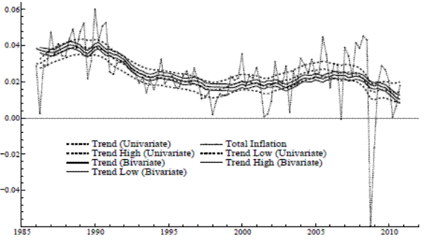
Figure 3: Observation weights for estimating trends in core inflation and total inflation for the local level model.

Figure 4: Gain functions.

Figure 5: Trend estimates, Bivariate Smooth Trend Model, for core and total PCE inflation.

Figure 6: Trend estimates, Univariate and Bivariate Smooth Trend Model, for total PCE inflation.

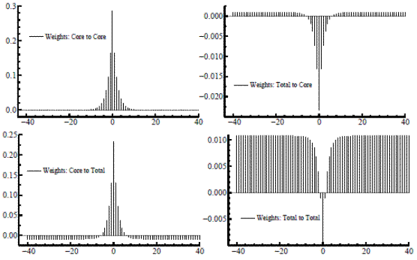
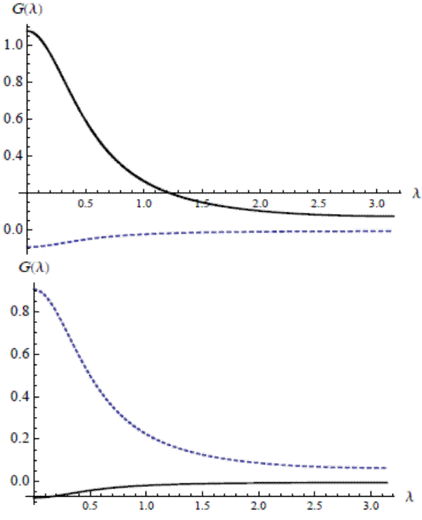
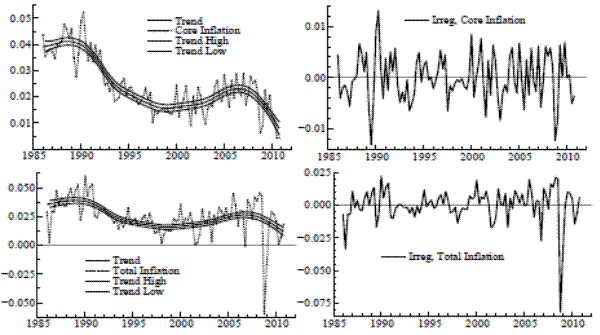
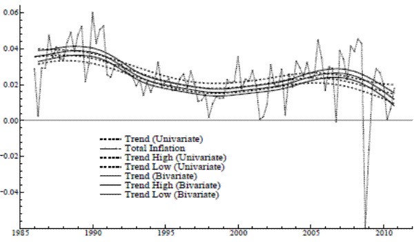
Figure 7: Observation weights for estimating trends in core and total inflation for the smooth trend model.

Figure 8: Gain functions.

Figure 9: Trend estimates, Bivariate Local Level and Smooth Trend Model, for total PCE inflation.

Footnotes

1. This encompasses processes that are nonstationary only in second moments after appropriate differencing; that is, they are nonstationary only in levels and may have heteroskedastic disturbances. Return to Text

2. For some non-Gaussian distributions, the optimal signal estimator can be computed with simulation techniques. See Trimbur (2010) for an example with an irregular distributed as a Student-t. However, explicit formulas are not available for most non-Gaussian distributions. Return to Text

3. As an aside, we independently estimated all the models using (12) and our matrix expressions for $\Sigma _{\mathbf{w}}$ , and obtained nearly identical results. Note that, as shown in Bell and Hillmer (1991), a state space likelihood corresponds to the Gaussian likelihood under Assumption $% M_{\infty }$ if it is initialized using the transformation approach of Ansley and Kohn (1985); other initializations, such as the diffuse, can produce different results. Return to Text

^♣ This version is optimized for use by screen readers. Descriptions for all mathematical expressions are provided in LaTex format. A printable pdf version is available. Return to Text