
Why the Geographic Variation in Health Care Spending Can't Tell Us Much about the Efficiency or Quality of our Health Care System
Keywords: Geographic variation, medicare spending, health spending, Dartmouth
Abstract:
This paper examines the geographic variation in Medicare and non-Medicare health spending and finds little support for the view that most of the variation is attributable to differences in practice styles. Instead, I find that socioeconomic factors that affect the need for medical care, as well as interactions between the Medicare system, Medicaid, and private health spending, can account for most of the variation in Medicare health spending. Furthermore, I find that the health spending of the non-Medicare population is not well correlated with Medicare spending, suggesting that Medicare spending is not a good proxy for average health spending by state. Finally, there is a negative correlation between the level and growth of Medicare spending; low-spending states are not low-growth states and are thus unlikely to provide the key to curbing excess cost growth in Medicare.
The paper also explores the econometric differences between controlling for health attributes at the state level (the method used in this paper) and controlling for them at the individual level (the approach used by the Dartmouth group.) I show that a state-level approach is likely to explain more of the state-level variation associated with omitted health attributes than the individual-level approach, and argue that this econometric differences likely explains most of the difference between my results and those of the Dartmouth group.
More broadly, the paper shows that the geographic variation in health spending does not provide a useful measure of the inefficiencies of our health system. States where Medicare spending is high are very different in multiple dimensions from states where Medicare spending is low, and thus it is difficult to isolate the effects of differences in health spending intensity from the effects of the differences in the underlying state characteristics. I show, for example, that the relationships between health spending, physician composition and quality are likely the result of omitted factors rather than the result of causal relationships.
1 Introduction
It is well known that Medicare spending per beneficiary varies widely across geographic areas. The conventional wisdom from the leaders in this research area, the Dartmouth group, is that little of this variation is accounted for by variation in income, prices, demographics, and health status, and, instead, most of the variation represents differences in "practice styles." Further, the Dartmouth research suggests that the additional health spending of the high-spending areas does not improve the quality of health care, and, indeed, might even diminish it.
One of the implications of the Dartmouth work is that health care spending can be reduced without significant effects on health outcomes. For example, Sutherland, Fisher, and Skinner (2009) argue "Evidence regarding regional variations in spending and growth points to a more hopeful alternative: we should be able to reorganize and improve care to eliminate wasteful and unnecessary service." The Dartmouth group has also argued that this geographic variation holds the key to reducing excess cost growth in health care. According to Fisher, Bynum, and Skinner, (2009), "By learning from regions that have attained sustainable growth rates and building on successful models of delivery-system and payment system reform, we might...manage to "bend the cost curve." ....... Reducing annual growth in per capita spending from 3.5% (the national average) to 2.4% (the rate in San Francisco) would leave Medicare with a healthy estimated balance of $758 billion, a cumulative savings of $1.42 trillion."
In this paper, I reexamine the geographic variation in health spending and find little support for the Dartmouth views. I find that, rather than reflecting differences in practice styles, most of the geographic variation in Medicare spending likely is attributable to differences in socioeconomic factors that affect the need for medical care, as well as to interactions between the Medicare system, Medicaid, and private health spending. I also find little correlation between the health spending of the non-Medicare population and that of the Medicare population, suggesting that Medicare spending is not a good proxy for average health spending by state. Finally, I find that there is a negative correlation between the initial level and subsequent growth of Medicare spending; low-spending states are not low-growth states and are thus unlikely to provide the key to curbing excess cost growth in Medicare.
More broadly, the paper shows that the geographic variation in health spending does not provide a useful measure of the inefficiencies of our health system. States where Medicare spending is high are very different in multiple dimensions from states where Medicare spending is low, and thus it is difficult to isolate the effects of differences in health spending intensity from the effects of the differences in the underlying state characteristics. I show, for example, that the relationships between health spending (both Medicare and non-Medicare), physician composition, and quality are likely the result of omitted factors rather than the result of causal relationships. Insights into the relationship between health spending and outcomes are more likely to be provided by natural experiments such as that analyzed by Doyle (2007), who showed that among visitors to Florida who had heart attacks, outcomes were better at hospitals with higher spending, or the true experiment run in Oregon in which a group of uninsured low-income adults was selected by lottery to be given the chance to apply for Medicaid (Finkelstein et al, 2011).
The paper is organized as follows. First I present the basic results from the Medicare regressions, and show that the cross-state variation in average Medicare spending is well explained by differences in population characteristics across states. I then compare my results to those of the Dartmouth group and suggest a number of reasons why my results differ. In an appendix, I show that, econometrically, there is a difference between controlling for attributes at the individual level (the Dartmouth approach) and controlling for them at the state level (the approach used here), and that this difference is likely to be empirically important when it comes to health care. I argue that my state-level approach better controls for the variation in health and other socioeconomic variables that affect health demand.
I then explore the relationships between Medicare and non-Medicare spending across the states, and show that the two are not particularly correlated, and thus Medicare is not a good proxy for total health spending by states. This lack of correlation is quite important in thinking about the relationship between provider workforce characteristics, quality, and health spending. In particular, I show that taking into consideration some of the demographics and health insurance variables by state changes the conclusions one gets from previous studies. Finally, I show that the growth rates of Medicare spending are negatively related to the level of health spending-that is, low spending states tend to have higher growth rates than high-spending states. The conclusion assesses the implications of this work for Medicare policy.
2 Data
The main data source is the CMS national health accounts, which provide a breakdown of total health spending across states by payer and service. These data are supplemented by a wide variety of state-level data on income, health insurance status, health behaviors, social capital, and demographics. The sources for these data are included in Appendix 2.
This study focuses on the level of "acute" health spending - that is spending on hospitals, physicians, and other professionals, and omits spending on long-term care, dental care, and prescription drugs. "Acute" health spending, which accounted for 85% of Medicare spending and 65% of total health spending in 2004, is what analysts typically have in mind when discussing physician practice styles. Long-term care, which accounts for much of the remaining Medicare spending, will be driven in important ways by both social factors (do you move in with children) and Medicaid and other public policies across the states and thus excluding these expenditures will ease the analysis.1
The focus on acute spending makes comparisons between Medicare spending and spending for the non-Medicare population easier as well, as they are much less likely to use long-term care. I use both the CMS state health accounts and private health insurance premiums from the Medical Expenditure Panel Survey to measure non-Medicare spending. The empirical work in this paper uses data from 2004, but the results are quite similar for earlier years.
3 The Geographic Variation in Medicare Spending
The Dartmouth group has documented the wide variation in per-beneficiary Medicare spending across the states. As shown in the first column of Table 1, Medicare spending on acute health care (hospitals, physicians and other professionals) ranged from a low of $4,729 (in New Mexico) to a high of $7,521 (in Maryland ), with a standard deviation of $711.
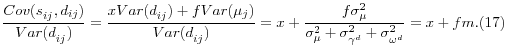
As first noted by Cutler and Sheiner (1999), much of the cross-state variation in real Medicare spending can be explained, in an econometric sense, by differences in the average health of the population. Figure 1, for example, shows the close correlation between a state's obesity rate and its real per beneficiary Medicare spending.2 The figure shows that, at least for the variation in Medicare spending by state, there is a systematic relationship between population characteristics and spending. Thus, what have been deemed "practice style" differences are not randomly distributed, but, rather, closely related to the environment in which physicians practice. That is, states with similar demographic characteristics have similar levels of real Medicare spending.3
Table 2 reports the results of regressions of acute Medicare spending on state characteristics. In these regressions, state per capita income is included to control for variation in prices across states.4 As shown in column 1, the combination of per capita income and age distributions explains only about 30 percent of the variation in acute Medicare spending across states. However, including measures of health-in particular, the obesity rate in the state and the percent sedentary, increases the explained share of spending to 48 percent.5 Adding in the percent uninsured raises the explained share of spending to 75 percent, and adding in the percent black raises it to 81 percent.
Turning back to Table 1, we can see how the variation in health spending changes once these factors are accounted for. As noted in the far right column, including age, income, health and other demographic factors lowers the standard deviation from $711 for the unadjusted spending to just $289
for the adjusted spending. Figure 2 plots the adjusted Medicare spending (in logs) against the log of unadjusted Medicare. It shows that, while adjusted and unadjusted spending are correlated, the relationship is fairly weak (the coefficient on unadjusted Medicare spending is .16 and the
R![]() is .14). Many states that appear to be high-cost, like Florida and Connecticut, no longer are once the demographic and health variables are included; similarly, Utah, Idaho, Montana,
Vermont, and Maine, which are on the low end of the distribution of unadjusted Medicare spending, appear to be relatively high spenders once the adjustments have been taken into account. These regression results suggest that the cross-state variation in Medicare spending is tightly associated with
the characteristics of state populations, and that, once these characteristic are controlled for, the variation in spending is fairly small.
is .14). Many states that appear to be high-cost, like Florida and Connecticut, no longer are once the demographic and health variables are included; similarly, Utah, Idaho, Montana,
Vermont, and Maine, which are on the low end of the distribution of unadjusted Medicare spending, appear to be relatively high spenders once the adjustments have been taken into account. These regression results suggest that the cross-state variation in Medicare spending is tightly associated with
the characteristics of state populations, and that, once these characteristic are controlled for, the variation in spending is fairly small.
Table 3 presents the information in a way that is more directly comparable to some of the work that has been done previously. For this table, states are sorted according to unadjusted Medicare spending, and then put into quintiles based on population shares (so that roughly 20 percent of the Medicare population is in each quintile.) The table shows how much of the variation in spending is explained by the covariates in Table 2. Comparing the top quintile to the bottom quintile, one can see that unadjusted spending is $1,990, or 38 percent higher, in the top quintile compared to the bottom quintile. Adjusted spending, however, shows much less of a variance, with the difference between the top and bottom quintiles averaging just $315, or 5 percent.
These results are markedly different from those presented in much of the recent literature. For example, in response to criticisms that the Dartmouth results reflect unmeasured differences in health and socioeconomic status, Sutherland, Fisher, and Skinner (2009) showed that even with such controls, most of the geographic variation remained. Using the Medicare Beneficiary Survey, which contains a richer set of health attributes than the Medicare data, they found that controlling for age, race, income, self-reported health status, presence of diabetes, blood pressure, body-mass index, and smoking history only eliminates about 30 percent of the difference between spending in the top and bottom quintiles.6 They conclude that "more than 70% of the differences in sending that cannot be explained away by the claim that `my patients are poorer or sicker."'
However, it is important to remember this literature is focused on regression residuals, in the sense that all geographic variation that is not explained by the controls is labeled as variation in practice styles (the logic being that, if health spending varies across states independently from the needs of the patients, then the variation must be related to how patients are treated.) Thus, including only a few health measures in the equation-particularly when these measures do not explain a significant fraction of the within-state variation-does not alleviate the concern that there is still important omitted variation in underlying health and health needs. (I discuss below how state-level variables. like the state average obesity rate shown in Figure 1, better capture the effects of omitted health measures.)
Zuckerman, Waidmann, Berenson, and Hadley (2010), recognizing this, explored the effects of adding additional health measures as controls in the estimating equations. They controlled for whether the individual died that year, whether a number of conditions were newly diagnosed, and whether the individual had a history of heart attack, stroke, and a number of other conditions. In addition, they included information on supplementary health insurance. Including these other health factors explained an additional 7 percent of the difference between quintiles 1 and 5, so that 63 percent of the variation remained unexplained. As they note, however, even with their health measures, "they do not capture the severity of illness or the presence of multiple chronic conditions." Finally, a recent Medicare Payment Advisory Commission (2009) report found that including more detailed measures of beneficiary health reduces the geographic variation considerably. However, Skinner and Fisher (2010) point out that controls that depend on diagnoses of conditions may well control for the very variation that they are trying to explain. They note that "regions that have doctors who do more testing will have patients with more diagnoses and thus will appear to have sicker patients."
The Dartmouth researchers argue that their work adequately controls for the health of the beneficiaries in each state, and thus argue that it is something else that is causing this strong correlation between state attributes and spending. They argue that "social capital" plays a key role.7 Skinner, Chandra, Goodman, and Fisher (December 2008) notes that "physicians who live in ...high social-capital states are more likely to adopt new and effective innovations rather than simply performing more tests and procedures with questionable medical efficacy." For example, work by Skinner and Staiger (2007) demonstrates that states with high levels of social capital were more likely to follow recommended guidelines about prescribing beta blockers in the treatment of heart attacks.
Figure 3 shows that social capital is indeed highly correlated with real Medicare spending. However, as shown in Figure 4, social capital is also associated with the state variation in health and with race. Thus, it is possible that the association between social capital and Medicare spending is simply picking up the relationship between population health and Medicare spending; conversely, it is possible that the impact of the state health variables in the regressions shown in table 2 is being overstated because social capital is omitted. Table 4 compares these two possibilities. The table shows that social capital is a significant predictor of Medicare spending only when health variables are omitted from the equation.8 However, once these variables are included, social capital is no longer significant, suggesting that it is instead variation in population characteristics that accounts for the variation in spending, rather than variation in practice styles.
Thus, the regressions presented here suggest that most of the geographic variation in spending across states is explained by some very simple controls for race, demographic insurance status, obesity, and exercise. An obvious question is why these results differ from those done by the Dartmouth group and others?
Differences between state-level and individual-level approaches
The basic difference between the regressions in this paper and those used by the Dartmouth group and Zuckerman et al. is the level at which the health attributes were controlled for. The Dartmouth and Zuckerman work regress individual health attributes on individual spending, and then aggregates the residuals of these regressions by state. My work regresses average health spending by state against average health attributes in the state.
There are a number of important reasons why these approaches can yield different results. Most importantly, a state-level approach will yield different results if there is stronger correlation among health variables at the state level than at the individual level and if there are omitted health variables in the individual-level regressions. For example, suppose people are very health conscious in some states but less so in others. Further assume that in the non-health conscious states people tend to be obese and tend to smoke-but obese people in those states are not much more likely to smoke than non-obese people. Under these assumptions, including the average obesity in the state in a regression that does not include information about smoking will provide more information about the likelihood of smoking than including a person's obesity rate in an individual-level regression.
In general, if there is a state-specific factor that affects both measured and unmeasured health, a regression of mean health spending by state on mean health attributes by state will pick up more of the unmeasured health variation than a regression of individual health spending on individual health attributes. This proposition is proved formally in Appendix 1. However, it is worth examining some data to show that this is likely to be an important factor in explaining the differences between the Dartmouth results and the ones presented here. In order to do that, I use the microdata from the Behavioral Risk Factor Surveillance System (BRFSS), a telephone survey that asks about regular exercise, smoking, diabetes, obesity, self-reported health and insurance status.
Consider a data set that had information on an individual's exercise, smoking, poor health, diabetes, and insurance status, but not on obesity. How much better would state-level means of these variables do in explaining cross-state variation in self-reported health status than individual-level regressions? As show in Table 5, the answer is: much better.
The table compares the following methodologies. The "individual-level" approach uses the micro data to regress individual characteristics on the dependent variable. For example, in the first row of the table, the dependent variable is obesity and the independent variables are age, sex,
smoking, health status, diabetes incidence, and insurance status. I then calculate the mean residual of these regressions by state. This is similar to what Dartmouth does when it calculate the residuals of age-sex-and illness adjusted spending by state. The R![]() in the table is simply equal to 1 minus the ratio of the variance of the mean residuals divided by the variance of the mean obesity rates across the states. It measures the share of the cross-state variation that is
eliminated once the individual health attributes are controlled for.
in the table is simply equal to 1 minus the ratio of the variance of the mean residuals divided by the variance of the mean obesity rates across the states. It measures the share of the cross-state variation that is
eliminated once the individual health attributes are controlled for.
The methodology labeled state-level approach simply reports the R![]() from state-level regressions where the dependent variable is the mean obesity rate by state and the dependent
variables are the mean age, sex, smoking, health status, etc. by state. (Note that the data used in these regressions are identical to those used in the individual regressions; the only difference is that the regressions are of means by state.) This comparison is intended to mimic the difference
between my approach, which is based on state means, and that of the Dartmouth group, which does some adjustments to the underlying Medicare data before calculating state means.
from state-level regressions where the dependent variable is the mean obesity rate by state and the dependent
variables are the mean age, sex, smoking, health status, etc. by state. (Note that the data used in these regressions are identical to those used in the individual regressions; the only difference is that the regressions are of means by state.) This comparison is intended to mimic the difference
between my approach, which is based on state means, and that of the Dartmouth group, which does some adjustments to the underlying Medicare data before calculating state means.
As can be seen from the table, the differences in approaches are substantial. For example, 22 percent of the variation in obesity across states is explained by the individual-level approach, whereas 67 percent is explained by the state-level approach. Similar results are obtained when I switch the dependent and independent variables. While these regressions are only illustrative, they suggest that a state-level approach is likely to do a better job of controlling for omitted health variables.
In addition to the pure econometric difference between individual and state level regressions, some other factors may also contribute to the difference between my results and those of the Dartmouth group. First, the health and demographic variables used in the state-level regressions are not exactly the same as those that would be used in regressions of insurance and health status on individual spending. In particular, rather than being the health of the individual Medicare beneficiary, the health variables used here reflect mean population health including those not yet receiving Medicare. Thus, they might capture conditions that prevailed throughout a person's life. For example, sick patients are typically not obese, but if they had been obese throughout their life, this is likely to contribute to their current health status. Similarly, the health costs of diabetes depend on when a person first acquired the disease; in states where the incidence of diabetes is high (generally the states where obesity is high), diabetic Medicare beneficiaries are likely to be in worse health, on average, than in states where the incidence of diabetes is low. Similarly, all Medicare beneficiaries have insurance, but patients who did not have insurance prior to becoming eligible for Medicare are likely to be in worse health and to have greater need for health services. Thus, the average rate of uninsurance in a state may be a useful marker for patient health, even for those currently with insurance. An important advantage to using these state-level data is that they do not come from Medicare charts or from any encounter with the health system, and thus are not vulnerable to the charge that "people are more likely to be "diagnosed" with a disease when their physician or hospital treats them more intensively." (Skinner and Fisher, 2010)
Second, health systems may be geared toward the median or average patient. Physicians practicing in states with a sicker population may practice a more intensive form of medicine for all their patients than those practicing in states with a healthier population. For example, in states with sicker populations, hospitals may be more likely to invest in new technologies and physicians may be more likely to adopt more invasive procedures. Under this hypothesis, it is the mean-level of health needs that will determine medical expenditures, rather than the individual-level, and an approach based on state-means will do a better job of capturing the link between population health and Medicare expenditures.
Finally, in addition to capturing underlying population health, some of these variables might capture other attributes of the state that affect Medicare spending. For example, the share of the population that is uninsured could directly affect Medicare expenditures if providers are able to cost shift: they might perform more Medicare services or be more aggressive about Medicare billing in areas where the nonelderly population is uninsured.
4 Comparing Medicare and non-Medicare health expenditures
An important question is whether the geographic variation in Medicare spending is correlated with that of health spending as a whole. If Medicare is a good proxy for health spending in general, then studies reliant on Medicare data are likely to be quite informative about the health system as a whole. On the other hand, if the geographic variation in Medicare spending is not well correlated with that of non-Medicare spending, then drawing conclusions based on Medicare data becomes much more difficult: Not only would the conclusions from the Medicare studies not generalize, but a lack of correlation also raises important questions about the Medicare studies themselves. For example, if Medicare is not a good proxy for non-Medicare, this also one has to ask whether there are important interactions and spillovers between Medicare and non-Medicare that need to be taken into consideration when evaluating the Medicare variation. In addition, one has to be particularly careful when attempting to relate characteristics of the health system as a whole-for example, physician workforce characteristics-to Medicare expenditures, given that Medicare spending represents less than one-third of total health spending.
I define non-Medicare expenditures in two ways. The first method aims to capture all acute health spending received by non-Medicare beneficiaries. To do so, I calculate Medicare spending by service (hospital, physician and other professional) and "gross it up" to reflect total expenditures on behalf of Medicare beneficiaries, including deductibles and coinsurance.9 I then take total expenditures on hospitals, physicians, and other professionals by state, subtract the calculated Medicare expenditures, and divide the remainder by the non-Medicare population. This measure should reflect the average spending of the privately insured, the uninsured, and the Medicaid population (excluding dual eligibles). I label this measure non-Medicare acute spending. As noted by Skinner, Chandra, Goodman, and Fisher (2008), CMS uses a number of different sources to estimate health spending by state, as there is no single comprehensive source like there is with Medicare, and thus this variable likely is measured with a significant amount of error. Thus, as an additional check, I also examine the health insurance premiums by state from the Medical Expenditure Panel Survey (MEPS). These data represent private health insurance premiums, which provide another, independent, estimate of state variation in spending.
Table 6 examines the determinants of the cross-state variation in these two measures of health spending for the non-Medicare population. As shown in the first column, only the share of young people and per capita income explain the variation in MEPS premiums across states. As shown in the second column, these same factors affect non-Medicare acute spending in a very similar way; in addition, health spending for the non-Medicare population is lower the lower is insurance coverage, the more black the population is, and the higher the share urban. It is somewhat surprising that the health variables-obesity and sedentary-do not predict spending for the non-Medicare population whereas they were important for Medicare spending. This is likely due to a combination of factors, including the fact that less of the health spending of the non-elderly is related to underlying poor health (and more to childbirth, preventative care, accidents, and random health shocks), those in poor health are less likely to have insurance, and the effects of poor health on spending probably cumulate over time and have much less of an impact on health spending at younger ages. In addition, some of the variation in spending across states reflects price variation (likely reflecting the competitiveness of the health provider and insurance markets), which would not be affected by health status,
As shown in the third column of Table 6, there is a strong relationship between non-Medicare health spending and the MEPS premium. This is partly due to the fact that both measures are affected by population age and income. But, as shown in column 4, even controlling for these factors, the two measures are still correlated. The findings in Table 6 suggest that the non-Medicare acute spending measure is likely to be a reasonable measure of health spending for the non-Medicare population: it is correlated with private health insurance premiums, but also affected in the ways one might expect by variables that are likely to affect health spending for the uninsured and those on Medicaid.
How does health spending for the nonelderly population compare with Medicare spending? As is evident from Figure 5, neither the MEPS premium not the non-Medicare acute spending is correlated with Medicare spending across states. (This lack of correlation between Medicare and non-Medicare spending was also noted by Cooper (2010)). These plots do not adjust for any characteristics that may affect Medicare spending and non-Medicare spending differentially. For this, we turn to Table 7.
The first three columns of the table explore the relationship between MEPS and Medicare spending. As shown in the first column, without any controls, there is a small positive relationship between MEPS and Medicare, although the R![]() of the regression is quite low. Adding in the factors that explain both MEPS and Medicare spending (column 3) increases the coefficient somewhat, although it is still quite low. The final three columns do the same analysis for non-Medicare acute
spending. Without controls, Medicare spending has no predictive power for non-Medicare spending. However, when all the controls are included in the regression, the relationship between Medicare spending and non-Medicare spending becomes positive and significant.
of the regression is quite low. Adding in the factors that explain both MEPS and Medicare spending (column 3) increases the coefficient somewhat, although it is still quite low. The final three columns do the same analysis for non-Medicare acute
spending. Without controls, Medicare spending has no predictive power for non-Medicare spending. However, when all the controls are included in the regression, the relationship between Medicare spending and non-Medicare spending becomes positive and significant.
Table 8 delves further into the differences and similarities between Medicare and non-Medicare spending by examining spending on hospital care separately from spending on physicians. The table shows a striking difference in the two. Even with only demographic controls, there is a strong relationship between Medicare and non-Medicare hospital spending. Including controls for health and insurance status raise the coefficient on the log of Medicare hospital spending to almost 1 - indicating that a 1 percent increase in Medicare hospital spending is associated with a 1 percent increase in non-Medicare hospital spending. In contrast, however, without controls Medicare physician spending is negatively related to non-Medicare physician spending; with controls of health and insurance status, the two appear to be unrelated. Chernew et al. (2010) obtain similar results when comparing Medicare spending to spending for those insured through large employers-inpatient hospital utilization was similar for Medicare and non-Medicare beneficiaries, but total spending was not.
The basic message from these regressions is that, without appropriate controls for demographic, insurance status, and health, Medicare and non-Medicare spending are not well correlated. Factors that increase Medicare spending-health variables, percent black, and percent uninsured-either have no effect on non-Medicare spending (health variables) or reduce it (percent black and percent uninsured). Thus, places with poor health, high rates of uninsurance, and a large black population-like Mississippi and Louisiana-have high Medicare spending and low non-Medicare spending. Conversely, places with the opposite characteristics-like Vermont and Minnesota-have relatively high non-Medicare spending and low Medicare spending. This can be seen quite easily in Figure 6, which plots the ratio of Medicare to non-Medicare spending against the share of the population uninsured (top panel) and the share of the population that is black (bottom panel).
An additional important consideration is the degree to which hospitals and physicians cost shift. Providers in areas with a lot of uncompensated care may be more aggressive in Medicare billing and may treat insured patients more intensively to help offset the costs of the uninsured. Glied (2011) and Hadley and Reschovsky (2006) find evidence of cost shifting for physicians. The evidence on hospitals is more mixed (Frakt, 2011). With these data run separately for hospitals and physicians (not shown), the share uninsured in a state raises Medicare physician spending but does not affect Medicare hospital spending; thus, if there is any cost-shifting, it is more likely at the physician level.
5 A reconsideration of the relationships between Medicare spending and physician workforce and Medicare spending and quality
The lack of correlation between unadjusted Medicare and non-Medicare spending has important implications for analyses of the relationship between health system characteristics and Medicare spending. If places where Medicare spending is high are not places where total health spending is high, then it is hard to know how to interpret studies that find strong relationships between Medicare spending and other attributes of the health system.
One possibility is that the measures of health spending for the non-Medicare population are not providing a good signal of underlying utilization-either because the data are not very accurate, or because the prices paid for services can vary across states. However, the finding that factors that are known to lower utilization, such as insurance status and race, have the expected effect on non-Medicare spending; and that, once these factors are controlled for, non-Medicare hospital spending and Medicare hospital spending do move together-suggests that the lack of correlation between Medicare and non-Medicare health spending is real, at least to the extent it is correlated with state characteristics such as insurance status and race. Thus, analyses of the relationship between Medicare spending and other health system characteristics need to take these factors into account.
5.1 Medicare spending and the physician workforce
One area where such controls prove to be important is in the relationship between Medicare spending and the mix of physicians by state. Baicker and Chandra (2004) show that places with a greater share of physicians who are general practitioners have significantly lower Medicare spending and significantly higher quality than places with a higher share of specialists. This is an interesting finding because it suggests an actual policy that one might follow to lower costs and improve quality. One consideration, however, is that the mix of physicians is likely to depend on the demand for services of the entire population. If the elderly use specialists at a different rate than the nonelderly, the mix of spending by the nonelderly and the elderly might affect the composition of the physician workforce. More generally, the strong dependence of Medicare spending on health and demographic variables suggests that studies that do not control for these factors could be misleading. Cooper (2009a) argues that the share of general practitioners is a marker for sociodemographic differences, but does not test the implications of controlling for these characteristics.
Table 9 suggests that the relationship between the composition of the physician workforce and spending is not as clear as suggested by Baicker and Chandra. The first column of the table reports the results from a regression of physician composition, income, and demographics on Medicare spending, similar to the regression run by Baicker and Chandra. Holding the number of physicians constant, there is a strong negative relationship between the number of general/family practitioners per 1000 population and the level of Medicare spending-the Baicker and Chandra result. However, once the rate of uninsured and the percent black are included in the regression, the relationship goes away. The next two sets of columns report the results when the dependent variable is non-Medicare spending. Here, the story is the opposite-the more general/family practitioners the higher is non-Medicare spending. Again, this result is greatly diminished, and insignificant, once other covariates are included. Finally, examining the MEPS data, one finds no relationship between the composition of the workforce and the health insurance premium.
5.2 Medicare Spending and quality
Table 10 considers the impact of including covariates in regressions that examine the relationship between spending and quality. Numerous studies from the Dartmouth group have argued that higher medical spending is associated with lower quality (see, for example, Skinner, Staiger, and Fisher (2006.) Cooper (2009b) however, examines total spending by state (note that this measure is highly correlated with non-Medicare spending) and concludes that more spending is instead associated with higher quality.
The quality measure used in these studies-the Jencks index-is a ranking of states based upon how well they comply with recommended guidelines. For example, the index includes measures of whether hospitals treat heart attack victims with beta blockers, whether patients get antibiotics in the recommended 24 hours before surgery, and whether ace inhibitors are appropriately prescribed for patients with heart failure.
One advantage of this index is that, unlike outcomes-based measures of quality, they do not need to be adjusted for differing health risks, because they are based upon standards of care that virtually all patients should receive. A disadvantage, however, is that because they are measuring relatively simple and agreed-upon processes of care, they may be biased toward finding a negative relationship between spending and quality. As demonstrated by Chandra and Staiger (2007) with respect to heart attack treatment, areas differ in the type of care they specialize in: areas that tend to treat heart attack victims surgically are worse at medical management and vice versa. Thus, for patients who need surgery, intensive areas are best and for patients who don't require surgery, less intensive areas are better. However, because the Jencks scale only includes measures of medical management (five of the twenty-three measures in the index relate to timeliness and appropriateness of aspirin, beta blockers, and ace inhibitors for heart attack victims), it will be biased toward showing higher quality for areas that practice less intensive forms of medicine.
Furthermore, the index also includes measures that likely depend on demographic and socioeconomic characteristics. For example, it includes measures of whether the population (not just Medicare beneficiaries) gets flu shots, whether women have mammograms, and whether diabetics get appropriate screening tests (biennial eye exams, lipid profiles, and blood sugar (HbA1c) tests). Whether individuals receive these types of services may depend on whether there are clinics nearby, whether they have easy access to transportation, whether they have the time or the ability to take off work for an appointment, whether they have insurance, etc., and are thus likely related to demographic characteristics.
Finally, it is difficult to determine the direction of causality between health spending and quality. It is well known that failure to follow many of the recommended guidelines included in the Jencks index will likely result in poorer outcomes for patients, more complications which need to be treated, and more readmissions. Thus, places with poor quality care of the type measured by the Jencks index, for whatever reason, are likely to have higher Medicare expenditures. Under this interpretation, it is true that improving quality will result in lower expenditures, but simply reducing expenditures won't in itself lead to an improvement in quality.
In any case, the question remains as to how sensitive the literature's conclusions on quality and spending are to the inclusion of health and insurance controls. The first column of Table 10 reproduces the result found in much of the literature-Medicare spending is higher in areas with low quality, according to the Jencks ranking. (This measure ranks states from 1 to 51, with 1 being the best-thus an increase in rank represents a decrease in quality.) However, similar to the findings for the effect of physician workforce composition, health spending for the non-Medicare population has the opposite effect on quality, with more spending leading to higher quality. This surprising finding (which was first reported by Cooper (2010b)) is evident in Figure 7, which plots Medicare and non-Medicare spending against the Jencks ranking. Turning back to Table 10, the second column shows that these results persist when per capita income is included in the equations. The third and fourth columns of Table 10 replace actual Medicare and non-Medicare spending with the residuals from the equations relating such spending to demographic, health, and insurance status (from the fourth columns of Table 2 and Table 6, respectively). These adjusted spending measures represent the Medicare and non-Medicare spending that is unexplained by differences in state characteristics. These measures have no statistically significant relationship to quality rankings, although the coefficient on adjusted Medicare spending is still positive and large.
Table 11 examines the robustness of the Baicker and Chandra (2004) finding that more generalists leads to higher quality. Here too, including the share uninsured and the share black, or including social capital, leads one to conclude that there is little relationship between the variation in physician composition across states and the variation in quality.
The point of these exercises is not to argue that there is no relationship between physician workforce composition and spending, or quality and Medicare spending, but that such relationships are very hard to tease out from cross-state differences in Medicare spending. As noted previously, states with high levels of Medicare spending are very different from states with low levels of Medicare spending, and they are different in ways that are likely to affect all dimensions of the health system. While including controls for these differences is helpful and important, it is sometimes difficult to know whether the controls are exogenous or endogenous. For example, it could be that Medicare spending is high in places with a large black population because such populations have a lower share of general practitioners, or it could be that Medicare spending is high in places with a lower share of general practitioners because such places have a large black population with high Medicare expenses. The finding that the relationships between non-Medicare spending, quality, and physician composition are opposite to those of Medicare spending suggest that there are important interactions occurring that are difficult to control for.
6 Growth Rates
Finally, it is important to consider the implications of these findings for analyzing the growth of Medicare spending across states. The Dartmouth methodology often examines changes in the level of Medicare spending over time-thus, for example, Skinner, Staiger, and Fisher (2006), compare dollar changes in Medicare spending with changes in heart-attack survival rates to argue that increased spending was negatively related to increased survival. Similarly, Baicker and Chandra examine the changes in the level of Medicare spending and changes in quality.
This methodology would make sense if the prices paid by Medicare and the health needs of the populations did not vary across states. But, to the extent that the variation in the level of spending is associated with state attributes, a better approach is to compare the growth rates of spending across states.10 Otherwise, high-spending states with the same growth rate as low-spending states will appear to have increased spending more, thus making it more likely to find that increased spending is not worth it.11
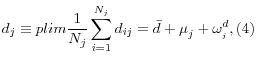
Furthermore, part of the message from the Dartmouth researchers is that low-cost areas are also areas that are more likely to adopt cost-effective technologies and less likely to adopt expensive technologies that don't increase quality. So, are low-spending states also low-growth states?
Figure 9 examines changes in relative Medicare spending over time. As shown in the top panel, the ranking of state Medicare spending has been fairly stable. However, as shown in the bottom panel, there is a strong negative correlation between health spending growth and initial level of health spending. Low-spending states tend to increase spending at a faster pace than high-spending states. For example, Medicare spending rose at an average rate of 6.3 percent per year in Idaho, but only 3.7 percent per year in Pennsylvania.
Table 12 reports the results from a simple regression of health spending growth on the initial spending level (growth in per capita income and insurance were not significant and are not included). The negative correlation between the level of health spending and the subsequent growth is observed from 1991 to 1997 and from 1997 to 2004. Thus, the data don't support the idea that low-spending states are low-growth states that adopt technology in a more cost-effective manner, and understanding regional variation is unlikely to be the key to figuring out how to "bend the cost curve."12
7 Conclusions
The evidence presented in this paper suggests that the variation in Medicare spending across states is attributable to factors that affect health and health behaviors, rather than practice styles. In addition, there are likely spillovers between Medicare and other health spending. Most importantly, states with large shares of their nonelderly population uninsured have lower non-Medicare spending and higher Medicare spending. This may be because lack of insurance before age 65 affects health status in ways that are not picked up by other measures, or because providers cost shift by finding ways to increase Medicare revenues to cover the costs of uncompensated care. Because of these interactions, it does not make sense to assume that the variation in Medicare spending captures the differences in health care resource utilization across states.
The paper also shows that conclusions about the relationships between health spending, physician composition, and quality are sensitive to the inclusion of variables like the share of the population uninsured, black, or obese. What this sensitivity demonstrates is the difficulty of using the geographic variation in spending for hypothesis testing. It is not surprising that states in the south spend more on Medicare and have worse outcomes. These states perform significantly worse in numerous areas, including high school graduation rates, test scores, insurance, unemployment, violent crime, and teenage pregnancy. There are many ways that such differences can affect health utilization and outcomes, including differences in underlying health, social supports and social stressors, patient self-care and advocacy, ease of access to services, capabilities and quality of hospital and physician nurses and technicians, and cultural differences in attitudes toward care. A comparison of health spending in Mississippi with health spending in Minnesota is not likely to provide a useful metric of the "inefficiencies" of the health system nor is it likely to provide a useful guide to improve the quality of care in places where it is lacking.
The evidence also suggests that low-cost states are not low-growth states. Thus, the geographic variation in Medicare spending is probably not the key to finding ways to slow spending growth while continuing to improve quality over time.
Finally, this paper also explores the differences between state-level and individual-level regressions. I show that, when there are omitted variables, the level at which the regressions are run matters. To the extent that one is focused on the unexplained portion of spending across states, running state-level regressions will do a better job of controlling for state-level characteristics than running individual-level regressions.
8 References
Baicker, Katherine and Amitabh Chandra. 2004. "Medicare Spending, The Physician Workforce, and Beneficiaries' Quality of Care." Health Affairs. W4-194, 7 April 2004.
Chandra, Amitabh and Douglas Staiger. 2007. "Productivity Spillovers in Health Care: Evidence from the Treatment of Heart Attacks." Journal of Political Economy. 115(1): 103-140.
Chernew, Michael E., Lindsay M. Sabik, Amitabh Chandra, Teresa B. Gibson, and Joseph P. Newhouse (2010). "Geographic Correlation between Large-Firm Commercial Spending and Medicare Spending." American Journal of Managed Care 16(2): 131-138.
Cooper, Richard, "States with More Physicians Have Better-Quality Health care," Health Affairs 28, no. 1 (2009a) w91-w102.
Cooper, Richard, "States with More Health care Spending Have Better-Quality Health Care: Lessons About Medicare," Health Affairs 28, no. 1 (2009b) w103-115.
Cutler, David M. and Louise Sheiner, 1999. "The Geography of Medicare," American Economic Review, American Economic Association, vol. 89(2), pages 228-233, May.
Finkelstein, Amy, Sarah Taubman, Bill Wright, Mira Bernstein, Jonathan Gruber, Joseph Newhouse, Heidi Allen, Katherine Baicker, and the Oregon Health Study Group, "The Oregon Health Insurance Experiment: Evidence from the First Year," NBER Working Paper 17190, July 2011.
Fisher, Elliott, Julie Bynum, and Jonathan Skinner, "Slowing the Growth of Health Care Costs-Lessons from Regional Variation, New England Journal of Medicine, 360: 849-852, February 26, 2009
Gawande, Atul, "The Cost Conundrum: What a Texas Town Can Teach us about Healthcare," The New Yorker, June 2009.
Hadley, Jack and James Reschovsky, "Medicare fees and physicians' Medicare service volume: Beneficiaries treated an services per beneficiary", Internal Journal of Health Care Finance Economics (2006) 6:131-150.
Jencks, Stephen, Edwin Huff, and Timothy Cuerdon, "Change in the Quality of Care Delivered to Medicare Beneficiaries, 1998-1999 to 2000-2001" JAMA, January 15, 2003.
Medicare Payment Advisory Commission. Report to the Congress: measuring regional variation in service use. Washington, DC: MedPAC, December 2009.
Skinner, Jonathan, Amitabh Chandra, David Goodman, and Elliott Fisher, "The Elusive Connection between Health Care Spending and Quality," Health Affairs, Web exclusive, 10.1377/hlthaff.28.1.w119, December 2008
Skinner, Jonathan, Douglas Staiger and Elliott Fisher, "Is Technological Change in Medicine Always Worth it? The Case of Acute Myocardial Infarction," Health Affairs, 25, no. 2. (2006):w34-w47.
Skinner, Jonathan and Elliott Fisher, "Reflections on Geographic Variations in U.S. Health Care," The Dartmouth Institute for Health Policy and Clinical Practice, May 12, 2010.
Sutherland, J.M, Fisher, E.S. and J.S. Skinner. 2009. "Getting Past Denial - The High Cost of Health Care in the United States." New England Journal of Medicine. 361(13): 1227-1230.
Zuckerman, Stephen, Timothy Waidmann, Robert Berenson, and Jack Hadley, "Clarifying Sources of Geographic Differences in Medicare Spending, The New England Journal of Medicine, 363:1, July, 2010.
Table 1
Cross-State Variation in Medicare Spending, 2004
| Acute Medicare Spending | No controls | Control for income and age groups | Control for income, age groups and health | Control for income, age groups, health, uninsured, and race |
| Average | $5,950 | $5,950 | $5,950 | $5,950 |
| Standard Deviation | $711 | $577 | $374 | $289 |
| Coefficient of Variation | 12% | 10% | 6% | 5% |
| Lowest | $4,729 | $5,016 | $5,089 | $5,041 |
| Highest | $7,521 | $7,269 | $6,734 | $6,538 |
| Range | $2,792 | $2,253 | $1,645 | $1,497 |
Note: The income, age group, health, uninsured, and race measures are the same as those in Table 2.
Table 2
Dependent Variable: Log Acute Medicare spending by state, 2004
| Log Per Capita Income | .31** | .55** | .63** | .53** |
| Log Per Capita Income (standard error) | (.11) | (.09) | (.08) | (.07) |
| Obesity Rate | .012** | .016** | .009* | |
| Obesity Rate (standard error) | (.006) | (.006) | (.005) | |
| Percent Sedentary | .01** | .009** | .006** | |
| Percent Sedentary (standard error) | (.003) | (.002) | (.002) | |
| Percent Black | .44** | |||
| Percent Black (standard error) | (.12) | |||
| Percent Uninsured | .011** | .010** | ||
| Percent Uninsured (standard error) | (.003) | (.003) | ||
| Share 65 to 74 | 3.8** | 3.2** | 2.0** | 1.0 |
| Share 65 to 74 (standard error) | (1.3) | (.8) | (.8) | (.7) |
| Share 75 to 84 | 8.5** | 7.7** | 6.5** | 5.5** |
| Share 75 to 84 (standard error) | (2.9) | (1.9) | (1.7) | (1.5) |
| Constant | .6 | -2.2 | -2.1* | -.05** |
| Constant (standard error) | (1.8) | (1.3) | (1.2) | (1.2) |
| R |
.27 | .69 | .75 | .81 |
| N | 48 | 48 | 48 | 48 |
** significant at 5% level; * significant at 10% level
Table 3
Most of the difference in spending by quintile is explained
| Quintile | Unadjusted Medicare Spending | Adjusted Medicare Spending |
| 1 | $5,258 | $5,850 |
| 2 | $5,964 | $5,922 |
| 3 | $6,311 | $5,955 |
| 4 | $6,731 | $6,146 |
| 5 | $7,248 | $6,165 |
| Difference between (5) and (1) | $1,990 | $315 |
States included in each quintile (based on Medicare enrollment):
- NM, UT, ID, MT, VT, ME, IA,SD, WY,NH,WI,OR,ND,WA,VA,CO,MN,AZ,AR
- NC,NE,IN,KY,RI,TN,SC,AL,WV,GA,MO,NV,KS
- OK,OH,MS,IL,PA
- CA,CT,MI,DE,TX,MA
- FL,LA,NY,NJ,MD
Table 4
Including Social Capital
Dependent Variable: Log Acute Medicare spending by state, 2004
| Social Capital | -.13** | -.05* | -.03 | .005 |
| Social Capital (standard error) | (.02) | (.03) | (.03) | (.03) |
| Log Per Capita Income | .40** | .53** | .61** | .53** |
| Log Per Capita Income (standard error) | (.08) | (.08) | (.08) | (.08) |
| Obesity Rate | .01* | .015** | .010* | |
| Obesity Rate (standard error) | (.005) | (.006) | (.005) | |
| Percent Sedentary | .007** | .007** | .006** | |
| Percent Sedentary (standard error) | (.003) | (.003) | (.002) | |
| Percent Black | 44** | |||
| Percent Black (standard error) | (.13) | |||
| Percent Uninsured | .010** | .011** | ||
| Percent Uninsured (standard error) | (.003) | (.003) | ||
| Share 65 to 74 | -2.0 | 1.3 | .90 | 1.2 |
| Share 65 to 74 (standard error) | (1.3) | (1.4) | (1.3) | (1.2) |
| Share 75 to 84 | -.09 | 4.8* | 4.8** | 5.8** |
| Share 75 to 84 (standard error) | (2.6) | (2.5) | (2.3) | (2.0) |
| Constant | 5.6** | .18 | -.6* | -.2 |
| Constant (standard error) | (1.6) | (1.9) | (1.8) | (1.6) |
| R |
.60 | .71 | .75 | .81 |
| N | 48 | 48 | 48 | 48 |
Table 5
Comparing Individual-level and State-level Approaches
BRFSS data
| Dep.endent Variable | Independent Variables | Share of State Variation Explained (1) Individual-Level Regressions | Share of State Variation Explained (2) State-Level Regressions | |
| 1. | Obesity | Smoker, Poor Health, Sedentary, Diabetic, Insurance Status, Age, Sex | .22 | .67 |
| 2. | Smoker | Poor Health, Obesity, Sedentary, Diabetic, Insurance Status, Age, Sex | .04 | .48 |
| 3. | Poor Health | Obesity, Smoker, Sedentary, Diabetic, Insurance Status, Age, Sex | .29 | .75 |
| 4. | Sedentary | Obesity, Smoker, Poor Health, Diabetic, Insurance Status, Age, Sex | .17 | .59 |
| 5. | Diabetes | Smoker, Poor Health, Sedentary, Obesity, Insurance Status, Age, Sex | .48 | .66 |
Table 6
Other health spending by state, 2004
| Dependent Variable | Log MEPS premium | Log Non-Medicare Acute | Log Non-Medicare Acute | Log Non-Medicare Acute |
| Log Per Cap Income | .19** | .35** | .27 | |
| Log Per Cap Income (standard error) | (.09) | (.14) | (.14) | |
| Log MEPS Premium | 1.0** | .41* | ||
| Log MEPS Premium (standard error) | (.22) | (.23) | ||
| Share of nonelderly population |
-2.2** | -2.2** | -1.2 | |
| Share of nonelderly population |
(.63) | (.93) | (1.0) | |
| Percent Sedentary | -.002 | .0 | ||
| Percent Sedentary (standard error) | (.002) | (.003) | ||
| Percent Obese | 0 | -.003 | ||
| Percent Obese (standard error) | (.005) | (.007) | ||
| Percent Black | .04 | -.24 | -.26* | |
| Percent Black (standard error) | (.10) | (.15) | (.15) | |
| Percent Uninsured | -.00 | -.01** | -.011** | |
| Percent Uninsured (standard error) | (.003) | (.004) | (.004) | |
| Percent Urban | -.03 | -.39** | -.38** | |
| Percent Urban (standard error) | (.08) | (.12) | (.11) | |
| Constant | 7.1** | 5.6** | -.35 | 2.6** |
| Constant (standard error) | (1.1) | (1.6) | (1.8) | (2.3) |
| R |
.48 | .65 | .29 | .67 |
| N | 48 | 48 | 48 | 48 |
Table 7
Relationship between Medicare and other health spending
| Dependent Variable | Log MEPS Premium | Log MEPS Premium | Log MEPS Premium | Log Non-Medicare Acute | Log Non-Medicare Acute | Log Non-Medicare Acute |
| Log Per Cap Income | .19** (.06) | .14 (.12) | .19* (.10) | .04 (.18) | ||
| Log Medicare acute spending | .15* | -.02 | .21 | .-.13 | -.17 | .48** |
| Log Medicare acute spending (standard error) | (.08) | (.07) | (.15) | (.15) | (.12) | (.21) |
| Share |
-2.1** | -1.6** | -4.6** | -2.3* | ||
| Share |
(.5) | (.7) | (.9) | (1.2) | ||
| Percent Sedentary | -.003 | -.004 | ||||
| Percent Sedentary (standard error) | (.002) | (.003) | ||||
| Percent Obese | -.003 | -.003 | ||||
| Percent Obese (standard error) | (.005) | (.005) | ||||
| Percent Black | -.04 | -.36* | ||||
| Percent Black (standard error) | (.12) | (.18) | ||||
| Percent Uninsured | -.001 | -.014** | ||||
| Percent Uninsured (standard error) | (.003) | (.005) | ||||
| Percent Urban | -4 | -.33** | ||||
| Percent Urban (standard error) | (4) | (.14) | ||||
| Share 65-74 | .44 | .8 | -4.5** | .2.3* | ||
| Share 65-74 (standard error) | (.67) | (.8) | (1.2) | (1.2) | ||
| Share 75-84 | 1.6 | 1.9 | -7.6** | -5.8** | ||
| Share 75-84 (standard error) | (1.5) | (2.0) | (2.6) | (2.9) | ||
| Constant | 6.9** | 6.3** | 4.8** | 9.1** | 14.1** | 8.6** |
| Constant (standard error) | (.7) | (1.0) | (1.9) | (1.3) | (1.7) | (2.7) |
| R |
.05 | .49 | .50 | 0 | .54 | .69 |
| N | 48 | 48 | 48 | 48 | 48 | 48 |
Table 8
Medicare vs non-Medicare: Hospitals and Physicians Services, 2004
Dependent Variable: Log Non-Medicare Spending by Service
| Hospitals | Hospitals | Physician | Physician | |
| Log Medicare | .36** | .97** | -.28** | .07 |
| Log Medicare (standard error) | (.18) | (.23) | (.10) | (.17) |
| Log Per Cap Income | -.14 | -.64** | .50** | .36* |
| Log Per Cap Income (standard error) | (.15) | (.19) | (.13) | (.19) |
| Share |
-4.3** | -4.2** | -4.0** | -1.4 |
| Share |
(1.4) | (1.2) | (1.1) | (1.8) |
| Percent Obese | -.02* | .013 | ||
| Percent Obese (standard error) | (.01) | (.009) | ||
| Percent Black | -.20 | -.66** | ||
| Percent Black (standard error) | (.26) | (.23) | ||
| Percent Uninsured | -.02** | -.013* | ||
| Percent Uninsured (standard error) | (.006) | (.007) | ||
| Share 65-74 | -6.2** | -3.6** | -1.0 | -1.4 |
| Share 65-74 (standard error) | (1.6) | (1.7) | (1.7) | (1.8) |
| Share 75-84 | -8.7** | -6.8** | -4 .0 | -7.9* |
| Share 75-84 (standard error) | (3.7) | (3.3) | (3.7) | (4.0) |
| Constant | 13.5** | 12.7** | 7.4** | 8.2** |
| Constant (standard error) | (2.8) | (2.9) | (2.4) | (3.1) |
| R |
.39 | .56 | .49 | .56 |
| N | 48 | 48 | 48 | 48 |
Table 9
Effects of Physician Workforce Characteristics on Spending
| Dependent Variable | Log Medicare Spending | Log Medicare Spending | Log Non-Medicare Spending | Log Non-Medicare Spending | Log MEPS Premium |
| General/Family Practitioners per 1000 | -.47** | -.04 | .56** | .23 | .05 |
| General/Family Practitioners per 1000 | (.13) | (.12) | (.10) | (.14) | (.06) |
| Total Physicians per 1000 | .01 | .01 | .06** | .04* | .03* |
| Total Physicians per 1000 | (.09) | (.02) | (.02) | (.02) | (.01) |
| Log Per Capita Income | .16 | .32** | .15 | .30** | .14 |
| Log Per Capita Income | (.14) | (.10) | (.11) | (.13) | (.07) |
| Percent Black | .80** | -.13 | |||
| Percent Black | (.13) | (.14) | |||
| Percent Uninsured | .01** | -.007* | |||
| Percent Uninsured | (.004) | (.004) | |||
| Share |
-.02** | -.01 | -.02** | ||
| Share |
(.01) | (.01) | (.01) | ||
| Percent Urban | -.003** | ||||
| Percent Urban | (.001) | ||||
| Share 65 to 74 | .01 | .002 | |||
| Share 65 to 74 | (.01) | (.01) | |||
| Share 75 to 84 | .04 | .04** | |||
| Share 75 to 84 | (.03) | (.02) | |||
| Constant | 5.2 | 3.4** | 6.6** | 5.4** | 7.3** |
| Constant | (2.4) | (1.7) | (1.1) | (1.4) | (.7) |
| R |
.41 | .69 | .60 | .69 | .52 |
| N | 48 | 48 | 48 | 48 | 48 |
Table 10
Relationship between Quality Ranking and Health Spending
Dependent Variable: Jencks Quality Ranking, 2000
| Log Medicare Spending | 58** | 86** | ||
| Log Medicare Spending (standard error) | (13) | (13) | ||
| Log Non-Medicare Spending | -64** | -40** | ||
| Log Non-Medicare Spending (standard error) | (13) | (12) | ||
| Log MEPS premium | -37 | |||
| Log MEPS premium (standard error) | (39) | |||
| Log Adjusted Medicare Spending | 38 | |||
| Log Adjusted Medicare Spending (standard error) | (29) | |||
| Log Adjusted non-Medicare Spending | -16 | |||
| Log Adjusted non-Medicare Spending (standard error) | (20) | |||
| Log Per cap Income | -51** | -22 | ||
| Log Per cap Income (standard error) | (12) | (19) | ||
| Uninsured | 2.2** | |||
| Uninsured (standard error) | (.4) | |||
| Sedentary | 1.5** | |||
| Sedentary (standard error) | (.2) | |||
| Constant | 25 | 116 | 559** | -84** |
| Constant (standard error) | (161) | (137) | (259) | (12) |
| Rsq | .51 | .66 | .07 | .66 |
| N | 48 | 48 | 48 | 48 |
Table 11
Effects of Physician Composition on Quality Ranking
Dependent Variable: Jencks Quality Ranking, 2000
| General/Family Practitioners per 1000 | -72** | -30** | -14 | 12 |
| General/Family Practitioners per 1000 (standard error) | (145) | (13) | (14) | (17) |
| Total Physicians per 1000 | -9** | 1 | .8 | .7 |
| Total Physicians per 1000 (standard error) | (3) | (2) | (2) | (2) |
| Percent Uninsured | 2** | 2** | 2** | |
| Percent Uninsured (standard error) | (.5) | (.4) | (.5) | |
| Percent Obese | 3** | 4** | 3** | |
| Percent Obese (standard error) | (.5) | (.5) | (.6) | |
| Percent Urban | 24** | 26** | ||
| Percent Urban (standard error) | (12) | (11) | ||
| Social Capital | -7** | |||
| Social Capital (standard error) | (2.7) | |||
| Constant | 85** | -66** | -101** | -88** |
| Constant (standard error) | (12) | (23) | (27) | (26) |
| Rsq | .35 | .70 | .72 | .75 |
| N | 48 | 48 | 48 | 48 |
Table 12
Growth Rates of Medicare Spending
| 1991-2004 | 1991-1997 | 1997-2004 | |
| Log Medicare Spending, 1991 | -.024** | -.028** | |
| Log Medicare Spending, 1991 (standard error) | (.005) | (.01) | |
| Log Medicare Spending 1997 | -.031** | ||
| Log Medicare Spending 1997 (standard error) | (.007) | ||
| Rsq | .34 | .10 | .28 |
| N | 48 | 48 | 48 |
Figure 1
Real Spending per Beneficiary and Obesity
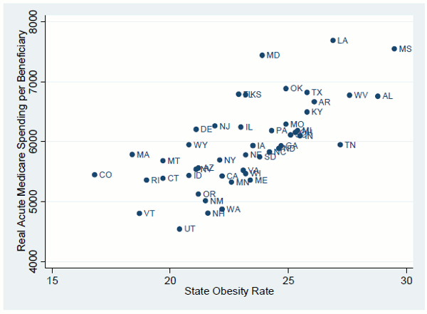
Figure 1 Data
Figure 2
Adjusted and Unadjusted Medicare Spending
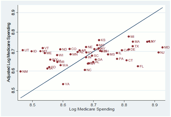
Figure 2 Data
Figure 3
Social Capital and Medicare Spending
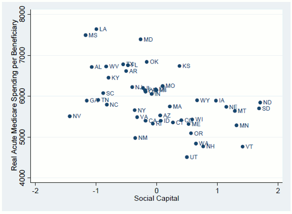
Figure 3 Data
Figure 4
Social Capital and Measure of State Health and Race
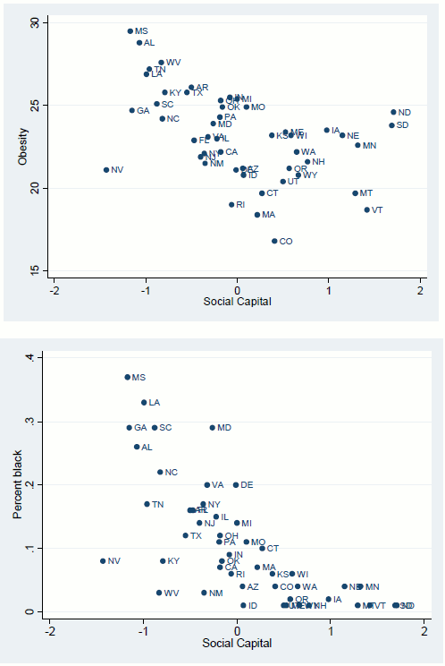
Figure 4 Data
Figure 5
Medicare and non-Medicare Spending
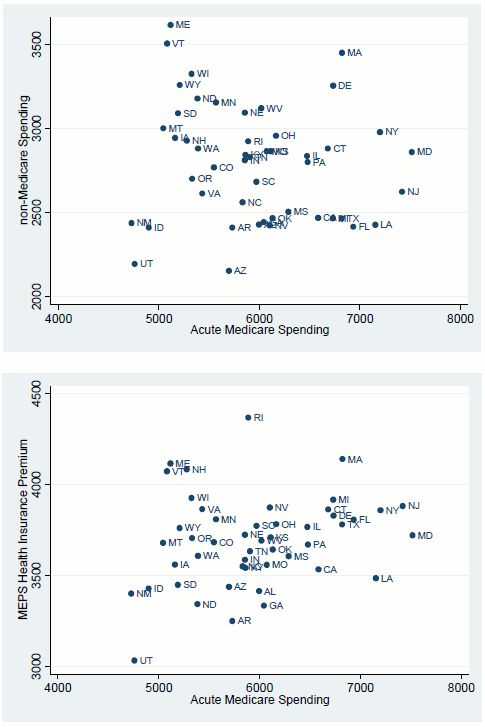
Figure 5 Data
Figure 6
Ratio of per-beneficiary Medicare acute to per-beneficiary non-Medicare acute Spending
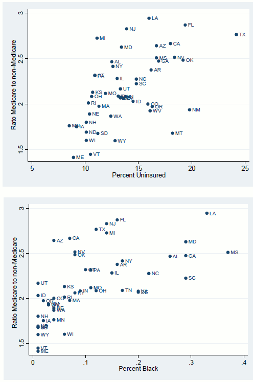
Figure 6 Data
Figure 7
Quality Rankings and Health Spending
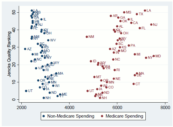
Figure 7 Data
Figure 8
Relationship between Adjusted and Unadjusted Medicare Spending and Quality
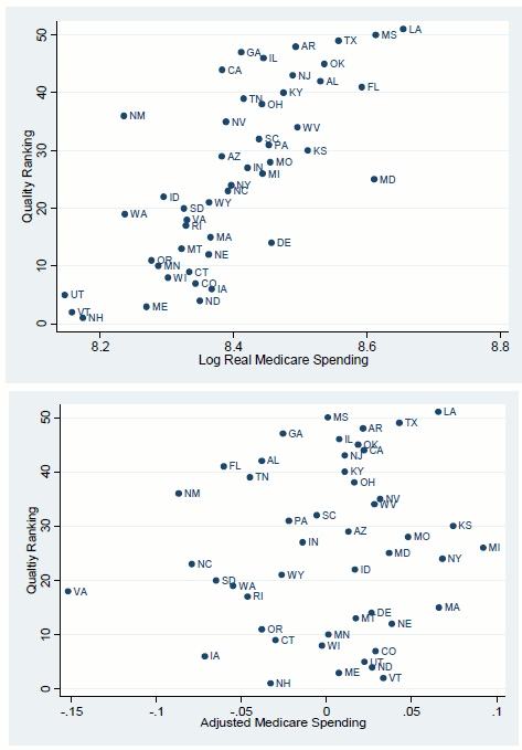
Figure 8 Data
Figure 9
Medicare Spending Growth
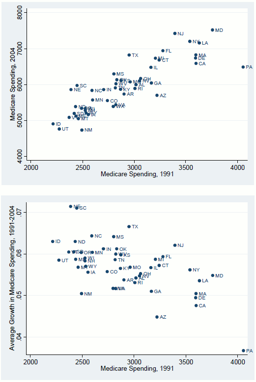
Figure 9 Data
9 Appendix 1
Potential Differences between State- and Individual- Level Regressions
As noted in the main text, regressions run at the state level have more power for explaining the variation in health spending and health attributes across states than regressions run at the individual level. In this appendix, I prove this formally by modeling the potential sources of health variation across the states, and I provide more detail on the empirical importance of this effect using data from the CDC's Behavioral Risk Factor Surveillance System (BRFSS).
The two approaches that I am comparing are the following:
- An individual-level approach: Regress individual health spending on individual health attributes. Compute the mean residuals of the regression by state. Determine the share of the variation in health spending across states that is explained by the regression.
- A state-level approach: Regress mean health spending by state on mean attributes by state. Compute the residuals of the regression. Determine the share of the variation in health spending across states that is explained by the regression.
I find that these two approaches can yield substantially different results if (1) some health attributes that could explain health spending are omitted from the health spending regressions, and (2) there are separate state-specific and individual-specific factors that affect the health attributes of individuals. Both of these conditions are likely to be met. First, it seems quite likely that analyses of individual health spending will omit some relevant patient characteristics, given the complicated nature of health spending and the limited data typically available. Second, the fact that mean health attributes vary substantially across states suggests that there are empirically-significant state-specific factors, because if all the variation were at the individual level, mean obesity, diabetes, and exercise, for example, would show no state variation.
To the extent that the two approaches do yield different results, the state-approach will explain more of the health-related variation than the individual approach, and thus provide a cleaner (but, under my framework, still imperfect) measure of variation in health spending that is unrelated to underlying health attributes ("practice styles.") Using the BRFSS, I show that, empirically, state-level regressions are likely to be substantially better than individual-level regressions at controlling for underlying health attributes that influence health spending.
A Model
Assume that health spending is a function of diabetes and smoking, but that only diabetes is observed. Then, to the extent that diabetes and smoking are correlated, the regression of health spending on diabetes will pick up some of the effects of smoking on health spending as well.
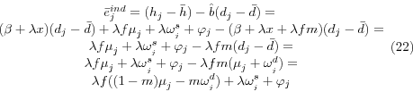
Diabetes and smoking could be correlated at the individual level if, for example, people with poor health habits tend to both smoke and have poor diets, or, conversely, if smokers tend to eat less.13 Diabetes and smoking could be further correlated at the state level if there is a third factor-say a state-specific attitude toward health behaviors-that affects both people's smoking decisions and diet decisions independently (so that a smoker in a state with poor health habits is no more likely to be diabetic than a non-smoker in that state). In the following, I model an individual's smoking as a function of being diabetic (so a diabetic has a different probability of smoking than someone without diabetes) as well as a function of a state-specific factor that independently affects both the decision to smoke and the likelihood of being a diabetic.
States are indexed by j = 1,....,N. The individuals in state j are indexed by (ij), i = 1,...,N![]() . An
individual's rates of diabetes, d
. An
individual's rates of diabetes, d![]() , and smoking, s
, and smoking, s![]() , have state-level and individual-level components.14 The rates are given by
, have state-level and individual-level components.14 The rates are given by
where the state-level components
![]()
![]() and
and
![]() are mean-zero random variables with respective variances
are mean-zero random variables with respective variances
![]() and
and
![]() These random variables are independent across states and independent of each other. They are also independent of state population size. Individual-specific
components
These random variables are independent across states and independent of each other. They are also independent of state population size. Individual-specific
components
![]() and
and
![]() are mean-zero random variables with variances
are mean-zero random variables with variances
![]() and
and
![]() They are independent across individuals, independent of each other, and independent of all state-level random variables. Inspection of equations (1) and (2) shows
that the coefficient from a regression of smoking on diabetes picks up two effects: the direction relation between smoking and diabetes at the individual level and the indirect relation at the state level. As is made clear below, the latter relation is obscured by an errors-in-variables problem,
which is more pronounced when the regression is run at the individual level than at the state level; it is this difference that leads to different results for state-level and individual-level regressions.
They are independent across individuals, independent of each other, and independent of all state-level random variables. Inspection of equations (1) and (2) shows
that the coefficient from a regression of smoking on diabetes picks up two effects: the direction relation between smoking and diabetes at the individual level and the indirect relation at the state level. As is made clear below, the latter relation is obscured by an errors-in-variables problem,
which is more pronounced when the regression is run at the individual level than at the state level; it is this difference that leads to different results for state-level and individual-level regressions.
Individual health spending is
As ![]() goes to infinity, means of health attributes and expenditures within state j are:
goes to infinity, means of health attributes and expenditures within state j are:
Assume that smoking and practice styles are both unobserved, and rewrite (3) as follows:
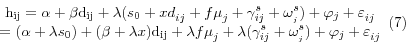
where
![]() ,
,
![]() and
and
![]()
Individual-level Regression
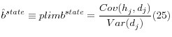
Consider the individual-level regression
Define
![]() as the probability limit of
as the probability limit of ![]() , the coefficient on diabetes
from (9). It is given by:
, the coefficient on diabetes
from (9). It is given by:
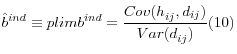
Given
![]()

Remember that diabetes is
![]() the error from the individual-level health spending regression is
the error from the individual-level health spending regression is
![]() and
and
![]() ,
,
![]()
![]()
![]()
![]() and
and
![]() are independent of all other random variables. Then,
are independent of all other random variables. Then,
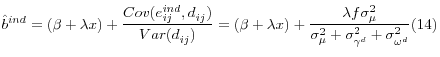
where
![]() and
and
![]() are the variances of
are the variances of
![]()
![]() and
and
![]() respectively.
respectively.
Define m as the share of the variance in diabetes rates that is explained by the state-specific variation common to both diabetes and smoking:
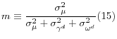
Note that ![]() is the probability limit of the coefficient from a regression of smoking on diabetes:
is the probability limit of the coefficient from a regression of smoking on diabetes:
When smoking is omitted, the coefficient on diabetes in a regression of health spending on diabetes picks up not only the direct effect of diabetes on health spending but also, because diabetes and smoking are correlated, part of the effect of smoking on health spending. The fm term has the same formulation as in a typical errors-in-variables model, where measurement error biases the estimated coefficient fm toward zero; in this model, the diabetes variable can be seen as measuring the true variable,
![]() with error.
with error.
The regression error from the health spending equation is:
Mean health spending nationally, ![]() is just
is just
Because
![]()
![]() and
and
![]() are all mean-zero and independent of all other random variables, the variance of
are all mean-zero and independent of all other random variables, the variance of
![]() -the variation in mean health spending that is unexplained by the individual-level regression-is just:15
-the variation in mean health spending that is unexplained by the individual-level regression-is just:15
State-level Regression
Now consider the regression of mean health spending by state on mean diabetes:
Given the independence of
![]()
![]() and
and
![]() ,
,
where z is defined as the share of the variance in mean diabetes rates that is explained by the state-specific variation common to both diabetes and smoking, so that
![]() ; hence,
; hence,
![]() Note that the equation for
Note that the equation for
![]() in equation (26) is the same as the equation for
in equation (26) is the same as the equation for
![]() in equation (16) except there is a z instead of an m. Also note that z
in equation (16) except there is a z instead of an m. Also note that z![]() m, because the variation in mean diabetes rates by state is smaller than the variation in diabetes rates across individuals. In particular,
m, because the variation in mean diabetes rates by state is smaller than the variation in diabetes rates across individuals. In particular,
where
![]()
The regression error
![]() from equation (24) is just:
from equation (24) is just:
which is identical to the mean error from the individual-level regression in (19), except for the difference between
![]() and
and
![]() . Thus, the variance of the residuals across states for the state-level regression is the same as in (23) above, except there is a z in place of an m.
. Thus, the variance of the residuals across states for the state-level regression is the same as in (23) above, except there is a z in place of an m.
Comparison between residuals of state-level and individual-level regressions
It is simple to show that state-level regressions always explain at least as much of the variation in health spending across states as individual-level regressions. Remembering that ![]() and that
and that
![]() so that
so that
![]() , we can write:
, we can write:
To solve this in terms of the fundamentals, we replace z and![]() :
:
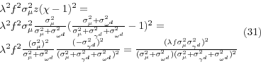
Thus, the variation in health spending by state that is unexplained by a regression of health spending on diabetes is larger in the individual-level regressions than in the state-level regressions under the following conditions:
-
 0 - smoking affects health spending
  0 - there is a state-specific shock to diabetes that also affects smoking
-
 0 - there is variation across states in this shock
 -
 0 - there is individual variation in diabetes that is unrelated to smoking
If any of these conditions are not met, then the individual-level approach has the same power as the state-level approach. The individual-level approach can never be better than the state-level approach. Intuitively, this makes sense as the individual variation in health attributes within a state can't help explain the variation in mean health spending across states-all it can do is add noise.
Appendix Figure 1 attempts to provide the intuition for this finding by showing the relationship between diabetes and smoking (which would then translate into the relationship between diabetes and health spending) under different assumptions about the state-specific shocks. In this example,
there are three states, state 1, state 2, and state 3. Mean diabetes varies by state. In the top panel, 1A,
![]() is greater than zero, meaning that there is a state-specific factor that affects both diabetes and smoking.16 The blue line shows the line of fit of the individual regression of smoking on diabetes, and the orange line shows the line of fit going of a regression of mean smoking on mean
diabetes. The orange line is steeper than the blue line, because the line of best fit in the individual regression is muted by the much weaker relationship between diabetes and smoking within a state.17 In contrast, in the bottom panel 1B,
is greater than zero, meaning that there is a state-specific factor that affects both diabetes and smoking.16 The blue line shows the line of fit of the individual regression of smoking on diabetes, and the orange line shows the line of fit going of a regression of mean smoking on mean
diabetes. The orange line is steeper than the blue line, because the line of best fit in the individual regression is muted by the much weaker relationship between diabetes and smoking within a state.17 In contrast, in the bottom panel 1B,
![]() is equal to zero, and there is no difference between the individual and the state regression.
is equal to zero, and there is no difference between the individual and the state regression.
B. Is This Empirically Important? Results from the Behavioral Risk Factor Surveillance System (BRFSS)
An examination of data from the Behavioral Risk Factor Surveillance System (BRFSS), a telephone survey of health habits and outcomes, provides a useful gauge of the likely empirical importance of this difference in omitted variable bias at the individual and state levels. Appendix 1 Table 1 compares the coefficients from state and individual-level bivariate regressions of five measures of health or health inputs: regular exercise, smoking, obesity, diabetes, and self-reported health. The top panel shows the results when regressions are run on individuals; the bottom panel shows the results when the regressions are of state means (of the identical data). State-level health measures are much more highly correlated than individual health measures. For example, the mean smoking rate in a state is a much better predictor of the mean poor health status than an individual's smoking is of his or her health status. A one percentage point increase in the rate of smoking in a state is associated with a .3 percentage point increase in the mean rate of poor health in a state; at the individual level, a 1 percentage point increase in the smoking raises the likelihood of poor health by only .02 percent. This discrepancy suggests that the state-level health regressions are likely to do a better job of picking up omitted health variables than the individual level regressions.
Table 5 in the main text of the paper provides further demonstration of the empirical importance of the difference between state level and individual level regressions. The table reports the results from regressions where one of the health variables is the dependent variable while the other health variables are the independent variables. For example, the first row of the table treats obesity as the dependent variable. The individual-level regression uses the individual as the observation, and regresses an individual's obesity on their other health measures. I then calculate the mean regression residual by state, and compare the variance of this mean residual (the part unexplained by individual health measures, or, equivalently, "individual-health-adjusted obesity") as a fraction of the variance of the mean obesity by state. This methodology mimics the Dartmouth methodology, where the Medicare expenditures of individuals are regressed against individual characteristics, and then residuals are calculated by state.18
The table shows that, in general, the state-level regressions have much more power than the individual-level regressions. For example, as shown in row 1, controlling for individual health variables other than obesity reduces the variance in mean obesity across states by 22 percent, whereas the state-level regression (where mean obesity is regressed against the means of the other health variables) explains 75 percent of the variance across states. This pattern holds regardless of which health variable is omitted. For example, while controlling for individual health attributes does nothing to explain the cross-state variation in smoking, including the state means of those variables explains 46 percent of it. (This is not surprising given that, at the individual level, smoking is negatively correlated with obesity and diabetes.) Similarly, the explained share of the cross-state variation in exercise increases from 17 percent to 59 percent, and the explained share of self-reported poor health increases from 29 percent to 75 percent, when going from individual-level to state-level regressions.
Thus, it is perhaps not surprising that the Dartmouth researchers find that controlling for individual health does not explain much of the variation in Medicare spending, whereas controlling for a state's health attributes (as in this paper) explains most of it.
Appendix Figure 1A: State-specific factor affects both diabetes and smoking 1B: State-specific factor affects only diabetes.
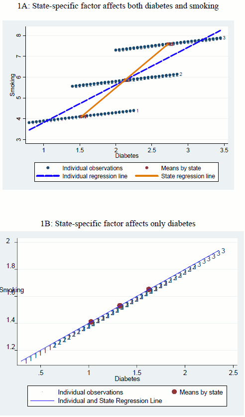
Figure A1a/A1b Data
Appendix 1 Table 1
Bivariate Regression Coefficients of Health Measures at Individual vs State Levels Regression of Individual Data (N = 178,698)
| Independent Variable: Poor Health | .07 | -.12 | .13 | .21 | |
| Independent Variable: Current Smoker | .02 | -.05 | -.04 | -.02 | |
| Independent Variable: Exercise Regularly | -.03 | -.06 | .07 | -.01 | |
| Independent Variable: Obese | .03 | -.05 | -.08 | .09 | |
| Independent Variable: Diabetes | .15 | -.06 | -.04 | .26 |
| Dependent Variable: Poor Health | Dependent Variable: Current Smoker | Dependent Variable: Exercise Regularly | Dependent Variable: Obese | Dependent Variable: Diabetes | |
| Independent Variable: Poor Health | .86 | -1.22 | .77 | .39 | |
| Independent Variable: Current Smoker | .34 | -.56 | .39 | .15 | |
| Independent Variable: Exercise Regularly | -.31 | -.35 | -.36 | -.16 | |
| Independent Variable: Obese | .45 | .58 | -.82 | .30 | |
| Independent Variable: Diabetes | 1.1 | 1.1 | -1.9 | 1.48 |
Appendix 2
Additional Data Sources
Uninsured by state: U.S. Census Bureau, Health Insurance Historical Tables (HIA Series)
Percent black: Population by Age: U.S. Census Bureau, Population by Sex, Race, and Hispanic Origin
Percent Urban (2000): U.S. Census Bureau, Urban and Rural Population by State, www.census.gov/compendia/statab/2012/tables/12s0029.xls
Obesity, Diabetes, No Exercise, Health Status, Smoking: CDC, Office of Surveillance, Epidemiology, and Laboratory Services, Behavioral Risk Factor Surveillance System, Prevalence and Trends Data
Per capita income: Personal income by state, U.S. Department of Commerce, Bureau of Economic Analysis
Social Capital: Bowling Alone.Com
Physicians by Specialty (2008), Kaiser State Health Facts http://www.statehealthfacts.org/index.jsp