
The Long and the Short of Household Formation*
Keywords: Household formation, headship rate, housing demand
Abstract:
One of the drivers of housing demand is the rate of new household formation, which has been well below trend in recent years, leading to persistent weakness in the housing market. This paper studies the determinants of household formation in the United States, including demographic and behavioral changes, and how they evolve over the long and short runs. There are three main findings: First, because older adults tend to live in smaller households, the aging of the U.S. population over the past 30 years has reduced the average household size, or equivalently, pushed up the headship rate and household formation. Second, after stripping out the effects of the aging population, the residual behavioral component of the headship rate has declined over time, thanks largely to rising housing costs. This shift has reduced household formation, all else equal. Finally, the short-run dynamics of headship and household formation reflect the effects of the business cycle. In particular, I find that poor labor market outcomes have played an important role in depressing the headship rate in recent years. Consequently, household formation could increase substantially as the labor market recovers and the headship rate returns to trend.
1 Introduction
In the wake of the housing bust of 2006 and the subsequent recession, the rate of new household formation in the United States plunged, and it has remained startlingly low since. Between 2006 and 2011, roughly 550,000 new households formed per year, on net, compared with 1.35 million per year over the previous five years. Indeed, household formation over the last five years appears to have been far lower than in any other five-year period over the 40 years for which we have annual data.1
Fewer new households formed has meant less demand for houses, leading to persistently low house prices and, in turn, a slump in new residential construction. Indeed, although data through the end of 2012 suggest that new housing starts and permits have begun to recover, they remain far below their long-run trends. This persistent weakness in the housing market has also contributed to the slow pace of the overall economic recovery. For example, the direct contribution of residential investment to annualized GDP growth sometimes reached 1 to 1.5 percent in recoveries prior to the mid-1980s. During the two years subsequent to the end of the recession in the second quarter of 2009, the contribution of residential investment to GDP averaged close to zero.
If some of the implications of low household formation are relatively clear, the underlying factors driving the individual choices that lead to household formation are much less so. Indeed, household formation involves a complicated series of decisions including, for example, whether to move out of a parent's home, whether to live alone or with roommates, and whether to get married to or form a partnership with another individual. In this paper, I analyze these choices and relate each to economic fundamentals, including the labor market, the cost of housing, and credit constraints.
Although a variety of labor and demographic studies are loosely related to to this paper, there has been relatively little academic work on household formation as such. Haurin et al. (1993) and Ermisch (1999) find that high rental costs retard household formation in the U.S. and U.K., respectively, and Haurin and Rosenthal (2007) find that lower headship rates also tend to reduce homeownership rates. Meanwhile, Kaplan (2012) shows that the option to move in with parents serves as insurance against labor market risk, while Dyrda et al. (2012) study the implications of such movements for aggregate labor supply. In contrast with most earlier work, my goal here is to provide a unified treatment of the determinants of household formation.
To understand these determinants, it is useful to examine the "headship rate", defined as the ratio of the number of household heads to the size of the adult population.2

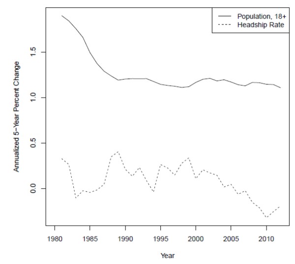
The aggregate headship rate, which is the reciprocal of the average number of people per household, determines the number of units needed to house a population of a given size.3 By taking logarithms and differencing equation 1, we can see that the (approximate) percentage change in the number of households is simply the sum of the (approximate) percentage changes in the adult population and the headship rate.
| (2) |
Figure 1 shows the 5-year percentage changes in the adult population and the headship rate. Although population growth has been by far the more important driver of household formation over the long run, most of the short-run variation in the growth rate of the number of households has come from shifts in the headship rate, particularly over the last decade. Consequently, this paper focuses on the determinants of the headship rate rather than immigration, fertility, or other factors affecting population growth.
I study these determinants in several steps. Since headship rates rise steadily over most of the life cycle, I first isolate and strip out the effect of the aging population, which has been pushing up the headship rate--or, equivalently, pushing down the average household size--since at least the 1970s. The residual behavioral component of the headship rate has actually drifted down over time, although it has fluctuated substantially at shorter frequencies.
Using multinomial logit models and decomposition techniques, I show that the trends in behavior over the period between 1980 and 2000 reflect rising housing costs, only partially offset by rising real incomes. I also show that the sharp decline in the headship rate from 2006 to 2010 is due in part to the rise in unemployment, confirming the intuition that the business cycle is helping to drive the shorter-run fluctuations in the data. I also find a small role for credit constraints in affecting household formation.4
Applying these insights, I estimate a fairly simple econometric model of the headship rate and then project it forward using the Congressional Budget Office's forecast of the unemployment rate through the end of the decade. Combined with ongoing population growth, this projection suggests that household formation could step up markedly as the labor market recovers. Indeed, as the headship rate returns to trend, the model predicts that household formation will rise to 1.6 million per year, substantially higher than its long-run average. While there are good reasons, detailed in section 7, not to take this precise figure too seriously, housing demand should receive substantial impetus from recovering household formation in the next several years.5
2 A Model of Headship
Although the aggregate headship rate--the ratio of households to people--is a simple concept, examining individual choices that affect the headship rate requires careful accounting. In particular, it is not always obvious whom to label as the "head" of a household, either theoretically or empirically. This section sets out a relatively simple dynamic model of headship that provides structure for the empirical work to follow.
Consider an adult in period ![]() with a set of characteristics (
with a set of characteristics (
![]() ), such as age, sex, and educational attainment. Provided she is neither out of the labor force (
), such as age, sex, and educational attainment. Provided she is neither out of the labor force (![]() ) nor unemployed (
) nor unemployed (![]() ), she earns her wage offer
), she earns her wage offer
![]() . She makes a choice
. She makes a choice ![]() among a set of four discrete living
states: Living with family members, such as her parents; living alone; living with a spouse or domestic partner; or living with non-relative roommates. Each state involves different utility benefits
among a set of four discrete living
states: Living with family members, such as her parents; living alone; living with a spouse or domestic partner; or living with non-relative roommates. Each state involves different utility benefits
![]() and housing costs
and housing costs
![]() . The chosen state may also involve a transfer payment
. The chosen state may also involve a transfer payment
![]() from other members of the household to compensate her for home production that benefits them, particularly if she does not work outside the home.
from other members of the household to compensate her for home production that benefits them, particularly if she does not work outside the home.
Her decision problem each year is
where
There are several other aspects of the model worth noting. First, it ignores the actual choice of where to live. Once a state is chosen, all housing units are identical, and individuals are indifferent between owning and renting. In a more complete model that explicitly considers the home ownership decision, an individual's credit score or foreclosure history may be relevant for headship decisions. I examine this possibility in the empirics.
Second, the choice of whether to enter the labor market is exogenous, and there is no search and matching process for finding a partner. In this model, an individual can immediately--though not necessarily costlessly--find a spouse or partner whose preferences regarding labor outside the home complement her own. For example, if she prefers to work and have a partner who concentrates on home production, she can always find one who is willing to do so in exchange for a transfer payment.
Finally, for completeness the model includes a cost of switching household states, which implies that the choice of a state today will be affected by the choice made yesterday. Rational individuals will thus take expected future conditions into account today. Since the data I use in this paper are cross-sectional, I do not allow for dynamics in the empirical work below, but the dynamic aspects of headship choice are deserving of further research.6
Mapping the decision problem in equation 3 into a headship rate requires specifying how each living state "contributes" to headship. Let
![]() be a function that maps states, conditional on characteristics, onto contributions. Since the point is to relate people to a household,
which by definition occupies one housing unit, the function is subject to the constraint that the contributions of all individuals in a household must sum to 1. For example, if each member of a married couple counts as half a head, then
be a function that maps states, conditional on characteristics, onto contributions. Since the point is to relate people to a household,
which by definition occupies one housing unit, the function is subject to the constraint that the contributions of all individuals in a household must sum to 1. For example, if each member of a married couple counts as half a head, then
![]() , regardless of characteristics. Alternatively, if heterosexual married men always count as the household head, as was the case in Census
data prior to 1980, then
, regardless of characteristics. Alternatively, if heterosexual married men always count as the household head, as was the case in Census
data prior to 1980, then
![]() and
and
![]() .
.
The particular choice of
![]() may depend on the data available or the empirical methodology chosen; I discuss several alternatives in the empirical section below. The key point is that once
a mapping is defined, we can calculate headship rates for different segments of the population. For example, we can define a headship rate for people of age
may depend on the data available or the empirical methodology chosen; I discuss several alternatives in the empirical section below. The key point is that once
a mapping is defined, we can calculate headship rates for different segments of the population. For example, we can define a headship rate for people of age ![]() by
by
3 Data
I draw on cross-sectional microdata from three sources: the Current Population Survey (CPS), the American Community Survey (ACS), and the decennial censuses. I use the Annual Social and Economic Supplement to the CPS, frequently referred to as the March CPS, to construct annual headship rates from 1980 through 2012.7 While the sample consists of less than 100,000 people, substantially fewer than the American Community Survey (ACS) or the decennial censuses, the CPS does ask the relevant questions about within-household relationships that I need to construct various headship measures. It also has the advantage of being available annually over a relatively long time span.
The second source of data is the ACS, an annual 1 percent sample of the U.S. population--approximately 3 million people--that includes detailed information on a variety of characteristics, including demographics, income, and employment status. Unlike the CPS, the ACS has a large enough sample to draw reliable inferences about patterns at the metropolitan level. Although versions of the ACS IPUMS8 are available from 2000 onwards, the survey was not fully implemented until 2006.9 Consequently, I use the 2006 and 2010 waves of the ACS to estimate headship models that shed light on the aftermath of the housing bust. Finally, to compare large samples over a longer time horizon, I use the 5 percent microdata samples from the 1980 and 2000 censuses.10
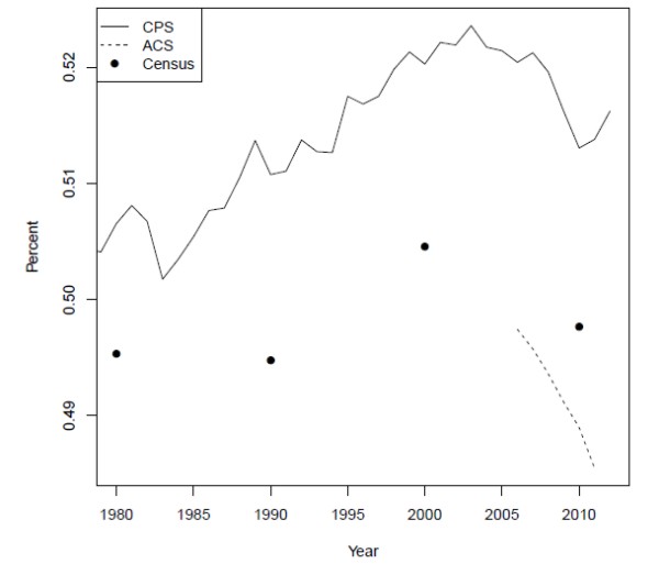
Although these surveys all have large samples and detailed publicly available microdata, they also provide strikingly different estimates of the headship rate. Figure 2 plots the aggregate headship rates from each sample, with the CPS represented by a solid line, the ACS by a dashed line, and the Census by solid circles. The CPS headship rate is markedly higher than both the Census and the ACS, which in principle could reflect the fact that the CPS excludes people in institutions, such as prisons or nursing homes, while the Census and ACS includes them. In practice, however, I have been unable to reconcile the estimates regardless of how the institutionalized population is counted. Regardless, the difference between the ACS and the Census in 2010, which is also sizable, cannot result from differences along this dimension.11
Importantly for my purposes, however, the trends in all of these series are broadly similar. For example, both census and CPS data show an increase in the headship rate from 1990 to 2000, followed by a decline back to roughly the 1990 level by 2010. The ACS, meanwhile, shows a relatively similar decline to the CPS in the latter half of the 2000s. Consequently, I draw on each data set for a different part of my analysis, while acknowledging concerns about their comparability. Specifically, I use the CPS to decompose annual movements in the headship rate from 1980 to the present. I use the microdata from the 1980 and 2000 censuses to compare longer run differences in behavior that affects headship and household formation. Finally, I use the 2006 and 2010 waves of the ACS microdata to examine the most recent decline in headship and household formation.12
3.1 Credit
One possible explanation for these declines is that borrowers have had less access to credit since the housing bust, both because banks are less willing to lend for a given set of borrower characteristics and because many borrowers now have foreclosures on their records. This suggests incorporating credit-related variables into the 2006-2010 comparison.
Importantly, the ACS lacks any information on credit-worthiness, other than income. In order to examine the effect of credit-related constraints on headship decisions, I use information from the FRBNY/Equifax consumer credit panel, which is a 5 percent random sample of credit-related information from all individuals with credit records and Social Security numbers.13 I focus in particular on individuals' credit scores and the presence of a foreclosure on their credit report.14 While the Equifax sample lacks any demographic information other than age, it does contain detailed geographic identifiers that make it possible to indirectly impute credit scores to individuals in the ACS.
This imputation is a two-step process. I first link individuals in the 2006 and 2010 waves of the credit panel to aggregate block and block-group level data from the 2000 Census. Within each year and public use microdata area (PUMA), I regress credit scores, foreclosure, and default on a nonlinear function of age and, given the demographics in the 2000 Census, the probabilities that an individual is of a given race, is of Hispanic origin, or has a given level of educational attainment. I then impute a credit score and probability of a prior foreclosure to each individual in the IPUMS using the resulting PUMA-level coefficients.15 Variation in imputed credit information thus comes from geography--the PUMA of the individual--crossed with his or her demographic characteristics and education.
Imputing credit in this way loses any idiosyncratic individual-level variation. This could be problematic if the effect of credit differs across the predictable and idiosyncratic components. Given the lack of large representative data sets with employment, income, and credit information, however, it is an improvement over existing work. In addition, the imputation process meets the criteria for the credit variables to serve as generated regressors (Wooldridge, 2002, p. 115), which means that--unlike when variables are measured with error--simple estimators remain consistent, although standard errors must be adjusted to account for the multi-stage estimation process.
4 The Role of Aging
Using the notation introduced in section 2, the aggregate headship rate in year ![]() can be decomposed into a weighted sum of headship rates by age, where the weights
are the fraction of the population at each age
can be decomposed into a weighted sum of headship rates by age, where the weights
are the fraction of the population at each age ![]() .16
.16
![\displaystyle HS_t = \sum_a \left[ HS_{a,t} \times \frac{P_{a,t}}{P_t} \right]](img24.gif) |
(4) |
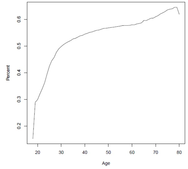
Over the life cycle, headship rates rise rapidly from less than 20 percent at age 18 to about 50 percent at age 30, then increase more gradually, as shown in figure 3. The substantial range of these estimates points to an important role for the age composition of the population: All else equal, an older population will demand more housing units, since older people tend to live in smaller households.
We can examine the effect of aging on the aggregate headship rate by defining a new aggregate that holds the headship rate for each age constant at its average value over time, while allowing the age profile of the population to vary.
![\displaystyle HS^D_t = \sum_a \left[ \overline{HS_{a}} \times \frac{P_{a,t}}{P_t} \right]](img25.gif) |
(5) |
Conversely, we can strip out the effects of aging and look at the underlying behavioral changes by holding the age profile constant but allowing the headship rates for each age to change.17
![\displaystyle HS^B_t = \sum_a \left[ HS_{a,t} \times \frac{\overline{P_{a}}}{\overline{P}} \right]](img26.gif) |
(6) |
Since the two components of the headship rate depend on age-specific headship rates, calculating them requires me to specify
![]() , the contribution of each living state to headship, conditional on characteristics. For the purposes of this paper, I assume
, the contribution of each living state to headship, conditional on characteristics. For the purposes of this paper, I assume
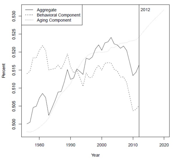
The dotted line in figure 4 shows ![]() , what the aggregate headship rate would have been in each year if the headship rate at each age had remained constant
at its average level over time while only the age distribution of the population had changed. The upward trend of this line indicates that the aging of the U.S. population has pushed up the headship rate substantially, or reduced the average household size. Census population projections, used to
extrapolate the aging effect into the future, imply that it will continue to do so at least through 2020. This demographic "push" explains why the aggregate headship rate--the solid line--has risen, on net, since the mid-1970s.
, what the aggregate headship rate would have been in each year if the headship rate at each age had remained constant
at its average level over time while only the age distribution of the population had changed. The upward trend of this line indicates that the aging of the U.S. population has pushed up the headship rate substantially, or reduced the average household size. Census population projections, used to
extrapolate the aging effect into the future, imply that it will continue to do so at least through 2020. This demographic "push" explains why the aggregate headship rate--the solid line--has risen, on net, since the mid-1970s.
After stripping out this the effects of aging, the behavioral component ![]() --the dashed line--appears to have declined over time. This decline suggests that there have been secular
shifts in the decisions of individuals within each age group that have increased the average household size. I examine the drivers of these secular shifts in the next section. Meanwhile, the behavioral component also shows sharp declines in the early 1980s, early 1990s, and late 2000s. These
declines and the subsequent recoveries suggest a role for the business cycle, which I explore in sections 6 and 7.
--the dashed line--appears to have declined over time. This decline suggests that there have been secular
shifts in the decisions of individuals within each age group that have increased the average household size. I examine the drivers of these secular shifts in the next section. Meanwhile, the behavioral component also shows sharp declines in the early 1980s, early 1990s, and late 2000s. These
declines and the subsequent recoveries suggest a role for the business cycle, which I explore in sections 6 and 7.
5 Behavioral Trends in the Long Run
To examine changes in individual behavior that affected the overall headship rate, I use decennial census microdata from 1980 and 2000. Table 1 contains the mean values of various attributes, broken out by year. The table indicates that the fractions of individuals who reported being unemployed or out of the labor force were similar in 1980 and 2000.19 The average real income was substantially higher in 2000, but so was the average rent, which I calculate for each metropolitan statistical area and impute to each household. In addition, both the education level and demographics of the population changed substantially: The fraction with a college education rose from 16 to 25 percent, while the fraction Hispanic nearly doubled and the average age increased by two years.20
To get a sense of how the characteristics in table 1 affect choices among the four living states I defined in section 2--with family, alone, with a spouse or partner, with a roommate--I estimate a multinomial logit model, pooling the observations from 1980 and 2000. This model can be thought of as a reduced-form implementation of the theoretical model in section 2, with the most important limitation being the lack of any dynamics, since the cross-sectional nature of the data do not allow for them.
The model includes log income, log MSA rent, and a series of indicator variables for unemployment, labor force participation, high school or college attendance, educational attainment, race, Hispanic origin, and sex.21 In addition, since some individuals report having very low, zero, or even negative incomes despite being neither unemployed nor out of the labor force, I define an additional indicator variable for incomes of less than $1,000.22 In order to flexibly control for the effects of the shifting age distribution over this period, I include B-splines for age and, because behavior among women at different ages shifted differentially relative to men, interact the splines with the female dummy. Finally, to control as best as possible for unobserved metropolitan characteristics, I include a full set of metropolitan fixed effects.
The marginal effects of the multinomial logit model, calculated at the covariate means, are shown in table 2.23 Each column represents one of the four possible living states, and each row one of the covariates. For example, all else equal, being unemployed raises the probability of living with family by about 4.5 percentage points, raises the probability of living alone by about 2 percentage points, and raises the probability of living with roommates by more than 3 percentage points. Since the probabilities in each row must sum to zero, being unemployed also necessarily reduces the probability of living with a spouse or partner by 10 percentage points.24
The estimated effects of the other covariates indicate that better education and better economic outcomes make individuals less likely to live with family or with roommates and more likely to live with a spouse or partner or to live alone. The only major exception to this broad pattern is that being out of the labor force is positively associated with being married, which is not surprising since one spouse may drop out of the labor force to concentrate on home production, such as raising children. The implications of the remaining covariate, rent, are also striking: A 20 percent increase in the average rent of an individual's MSA of residence, which corresponds to about one standard deviation of the log rent distribution, implies an increase in the probability of living with family of about 2 percentage points and a decrease in the probability of living with a spouse or partner of about 3.5 percentage points.25
The relationship between economic outcomes and living state, and thus headship, appears to be even stronger among the young. For example, table 3 shows that among adults between the ages of 18 and 30, being unemployed increases the probability of living with family by a full 9 percent, more than twice as high as in the population as a whole. The effects of higher MSA rents are also stronger. A 20 percent increase in rent raises the probability of living with family by about 3.5 percent and lowers the probability of being married or living with a partner by a slightly smaller amount.
These results indicate that a poor labor market or higher housing costs can depress headship and housing demand. We can examine the magnitude of the potential effects by using a nonlinear analogue to the standard Blinder-Oaxaca decomposition.26 The decomposition divides the change in an average outcome ![]() from time
from time ![]() to time
to time ![]() --for example, the probability that an individual
--for example, the probability that an individual ![]() lives alone--into two components,
lives alone--into two components,
where a bar indicates an average over individuals,
In the second line, the difference between the two terms containing ![]() is the portion of the difference in probabilities that can be explained by the model, while
is the portion of the difference in probabilities that can be explained by the model, while ![]() is the unexplained portion that arises from estimating
is the unexplained portion that arises from estimating ![]() on the pooled sample from
on the pooled sample from
![]() and
and ![]() .28 The third line comes from taking a first-order Taylor approximation of both
.28 The third line comes from taking a first-order Taylor approximation of both ![]() terms around the average covariate
across both years, with
terms around the average covariate
across both years, with ![]() denoting the approximation error. We can then further decompose the linearized "explained" part of the probability difference into portions attributable to each
covariate, simply by expanding the inner product in the third line, as follows:
denoting the approximation error. We can then further decompose the linearized "explained" part of the probability difference into portions attributable to each
covariate, simply by expanding the inner product in the third line, as follows:

This decomposition approach is similar to the one described in Yun (2004) for binary dependent variables. However, Yun (2004) creates weights by dividing each
![]() by the sum across all covariates,
by the sum across all covariates,
![]() . He then calculates the contribution
of each variable as its weight multiplied by the change in model-implied probabilities,
. He then calculates the contribution
of each variable as its weight multiplied by the change in model-implied probabilities,
![]() . In essence, he forces the contributions to sum to the total by parceling out the approximation error
(
. In essence, he forces the contributions to sum to the total by parceling out the approximation error
(![]() ) to each covariate according to its weight. This approach is substantially less attractive in a multinomial setting, because applying such a weighting scheme to each outcome yields
contributions that do not sum to zero for each covariate. Consequently, I prefer the approach in equation 8, which preserves this property but requires the approximation error to be accounted for separately.
) to each covariate according to its weight. This approach is substantially less attractive in a multinomial setting, because applying such a weighting scheme to each outcome yields
contributions that do not sum to zero for each covariate. Consequently, I prefer the approach in equation 8, which preserves this property but requires the approximation error to be accounted for separately.
The decomposition results for 1980 and 2000 are shown in table 4. The top two rows show the percentages of individuals who were in each living state in each year. During this period, the aggregate headship rate rose from roughly 49.5 to 50.5 percent, as shown in figure 2. The third line of the table, which shows the difference between the 1980 and 2000 percentages, demonstrates why: Adults became less likely to live with a spouse or partner or with roommates and correspondingly more likely to live alone. Under the assumptions about contributions to headship described in section 4 above, living with a spouse or partner or with a roommate contributes about 0.5 to headship.29 Consequently, a total reduction in these categories of about 2 percentage points and a corresponding increase in living alone implies the total increase in headship of about 1 percentage point that we observe in the data.
The line labeled "Total Explained" indicates the amount of each difference implied by the estimated effects from the multinomial logit model--table 2--and the changes in the covariate averages from 1980 to 2000, while the "Unexplained" line expresses the residual. This residual comprises changes in relevant covariates not included in the model as well as changes in the coefficients on those covariates between 1980 and 2000, since I pool the observations when I estimate the logit model. As the table shows, the changes in observables can explain most of the increase in the percentage living alone and the decrease in the percentage living with roommates. The model explains substantially less of the change in the percentage living with a spouse or partner, and it implies a modest decrease in the fraction living with family members, even though the actual change was close to zero.
The remaining lines of the table break down the "Total Explained" line into the contributions of each covariate and an approximation error that arises from using linear Taylor approximations to a nonlinear function.30 The contributions of unemployment, labor force participation, and individuals reporting zero income are all quite small, meaning that differences in the state of the business cycle were relatively unimportant in explaining the change in the headship rate between 1980 and 2000. Instead, the difference seems to be explained by the other categories, including the sum of the demographic effects, log income, log rent, and the sum of the education effects. Higher real income, better education, and changing demographics--especially the aging of the population--pushed down the fraction of individuals living with family and pushed up the fraction living with spouses or partners.
All of these effects imply higher headship rates, on net. In contrast, the increase in real rent of more than $1,500 per year--see again table 1--worked in the opposite direction, suppressing headship by lowering marriage and partnership rates, while simultaneously raising the fraction living with family members. These results suggest that the housing stock in desirable areas was not sufficiently elastic to accommodate all of the new households that would have resulted if real rents had remained flat (Glaeser et al., 2005; Quigley and Raphael, 2005). Instead, rent (and house prices) had to rise to equilibrate the housing market.
Although the model can explain some of the changes in behavior over this period, it fails to explain others. In particular, the model accounts for only about a fifth of the change in fraction living with a spouse or partner, even though the decline of 1.13 percentage points shown in the table understates the true change, because the 1980 data only count spouses and not partners. This result suggests that other changes in behavior, such as changes in preferences or other relevant covariates not included in the model, must have played an important role in holding down the behavioral component of the headship rate during this period.
6 Short-Run Dynamics
I now turn to examining changes in headship-related behavior between 2006 and 2010, a period in which the aggregate headship rate fell by more than half a percentage point, driven by a decline in the behavioral component. As shown in figure 4, the sharpest declines in both of these series occurred between 2008 and 2010, after the housing market had begun to collapse but roughly concurrent with the largest increases in unemployment.
Table 5 shows average attributes in the ACS over the two years. The fraction of the population that was unemployed increased by about 75 percent between 2006 and 2010, while the average real income fell. Meanwhile, the fraction of individuals with a foreclosure on their credit score, as imputed by the procedure described in section 3, more than doubled. Surprisingly, however, the average credit score actually increased slightly over this period, despite the foreclosures and other adverse credit events in the wake of the financial crisis.31 Finally, although house prices fell substantially during this period, the average MSA-level real rent increased, likely because rental units offered an alternative to former owner-occupants.
To focus on how these attributes affect headship choices, I estimate a multinomial logit model that parallels the one in the previous section. The marginal effects, shown in table 6, largely match my priors and are qualitatively similar to the results in section 5.32 For example, being unemployed implies a 7 percentage point higher probability of living with adult family members and an even larger decline in the probability of living with a spouse or partner. Similarly, individuals with lower incomes are more likely to live with family or with roommates and less likely to live with a spouse or partner.
As in the long-run results, higher rent in the individual's metropolitan area has a large effect on headship, with 20 percent higher rents--about one standard deviation--implying that individuals are about 3 percentage points more likely to live at home. They are about 2 percentage points each less likely to live alone or with with a spouse, and about 1 percentage point more likely to live with roommates. Meanwhile, the probability of being married rises and the probability of living with family falls with educational attainment, while high school or college attendance increases the probability of living with family.
The results in table 6 also suggest that credit availability affects headship. A one standard deviation increase in credit score raises the probability of living with a spouse by about 2 percentage point and reduces the probability of living alone by the same amount. In addition, a foreclosure raises the probability of living with family by 9 percentage points, thanks to reductions in living alone and with roommates.
While these credit results seem reasonably intuitive, the estimates for young adults reported in table 7 sow some doubt. As in the long-run results, most of the covariates, including unemployment and rent, have more impact on adults aged 30 or younger. The foreclosure effects, however, are both massive and seemingly at odds with the results for the whole population. Taken at face value, they indicate that a foreclosure increases the probability that a young adult lives with a spouse or partner by about 65 percentage points and decreases the probability he lives with family by more than 50 percentage points. This is almost certainly not a causal effect. Rather, individuals whom I impute to have a high likelihood of foreclosure also have a high probability of being married and a low probability of living with their families, simply because it is not possible to have a foreclosure on one's credit report unless one has owned a home. This line of reasoning suggests that all of the credit results should be viewed with some suspicion.
The decomposition of the living state probabilities shown in table 8 allows us to examine the implications of these estimates for the headship rate. The top two rows show the percentages of individuals who were in each living state in 2006 and 2010. The differences, shown in the third line, indicate that the decline in headship of about 0.8 percentage points during this period can be largely attributed to an increase in the fraction of individuals living with family. There was a roughly corresponding decrease in the fraction living with a spouse or partner.
The "Total Explained" and "Unexplained" lines indicate that the parameter estimates from the model and the change in covariates can explain roughly half of the change in each living state. Because the mean covariate values changed relatively little during this period, the approximation errors shown in the table are small. The most important covariates appear to be unemployment and metropolitan rent, which account for much of the explained portion of the changes in living with family and living with a spouse or partner. The rise in foreclosures also helps to explain the decline in headship, by accounting for a small boost to living with family and a corresponding decline in living alone.33
The effects of unemployment, higher rent, and foreclosure more than outweighed the higher headship that would have resulted from demographic change and better educational attainment. Interestingly, I find relatively small effects of school attendance. This result holds even in a decomposition of the decisions of young adults alone (not shown), suggesting that large numbers of young adults are not foregoing forming households in order to attend college or graduate school.
7 Projecting Household Formation
Given that unemployment seems to have depressed the headship rate in recent years, it is interesting to consider the possible paths of headship and household formation going forward, as the economy continues to recover. In this section, I use the insights from the microdata to construct a
relatively simple econometric model of the headship rate and use the model to project headship given the baseline labor market projection from the Congressional Budget Office. I first estimate a panel regression of headship rates, pooling across ages (![]() ) and years (
) and years (![]() ), on a linear time trend and the lagged unemployment gap (
), on a linear time trend and the lagged unemployment gap (![]() ).34 The trend captures the sort of long-run behavioral changes discussed in section 5, while the unemployment gap proxies for a variety of cyclical labor market conditions.35
).34 The trend captures the sort of long-run behavioral changes discussed in section 5, while the unemployment gap proxies for a variety of cyclical labor market conditions.35
As discussed above, a careful inspection of the data suggests that both the trend and cyclical pattern differ over the life cycle. In particular, unemployment has a stronger effect on headship among younger adults than among prime-age adults. Consequently, I allow the coefficients on the
unemployment gap and the trend to vary by age group,
![]() , with the groups defined as 30 or younger and 31 or higher:
, with the groups defined as 30 or younger and 31 or higher:
Note that modeling the headship rate at each age implicitly strips out the effects of the aging population on the aggregate headship rate, so the coefficients only capture the behavioral effects discussed above.36
Table 9 shows the estimated parameter values from equation 9.37 As suggested by the results above, young adults are quite sensitive to the business cycle, with each percentage point rise in the (aggregate) unemployment gap depressing the headship rate by 0.36 percentage points, relative to trend. By contrast, the headship rate of adults more than 30 years old drops by only 0.08 percentage points. The downward trend in headship has also been much stronger among younger adults.
These estimates, combined with the Census Bureau's population projections from 2012, allow me to predict the headship rate through 2020. I first calculate the fitted values of the headship rate at each age, given the time trend and the predicted unemployment gap from the CBO. I then aggregate the age-specific fitted headship rates using the Census Bureau’s projected population shares as weights, which reintroduces the effects of the aging population.
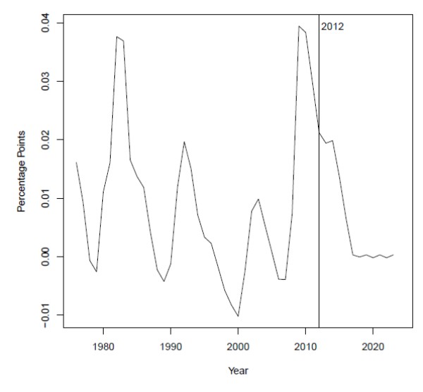
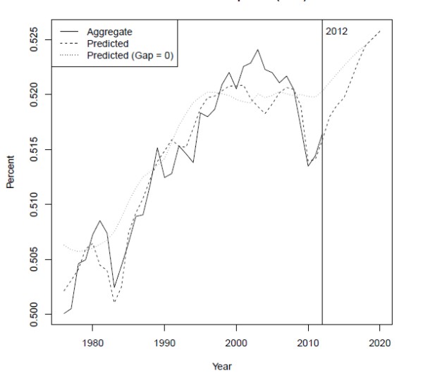
The headship projection depends crucially on the unemployment gap, which, as shown in figure 5, rose to about 4 percentage points in 2010 before declining over the last two years. Despite this decline, the CBO projects that the gap will remain elevated through 2014 before falling back to roughly zero in 2017. Figure 6 plots the aggregate headship rate, the predicted headship rate given the unemployment gap projection, and the predicted headship rate when the unemployment gap is set to zero over the whole horizon. The model fits the data reasonably well, and it clearly demonstrates the important role of the unemployment gap in depressing household formation. Indeed, if the unemployment gap had been zero in 2011--the dotted line--the model predicts that the headship rate would have been more than half a percentage point higher, which translates to an additional 1.5 million households.
The other notable feature of the chart is that, while the headship rate remains below trend for some time, the model implies that it should rise fairly rapidly. This projected recovery follows the small increases in the headship rate realized over the past two years, a feature of the data that the model fits rather nicely. The increase reflects the aging of the population and the (slow) projected decline in the unemployment gap. As the "headship gap" closes, the model implies that household formation should rise above its trend pace, as younger adults begin to move out of their parents' homes, for example.
Given the predicted headship rate, the predicted pace of household formation depends on aggregate population growth. Between the 2000 and 2010 Censuses, the adult U.S. population grew by about 25 million, or 2.5 million per year. The Census Bureau projects that average population growth from 2012 through 2020 will be somewhat slower, about 2.2 million per year. Even if the headship rate were to remain flat at its 2012 level of about 51.5 percent, we would thus expect new household formation of 1.1 to 1.2 million per year, substantially higher than in recent years.38 If the headship rate follows the model projection from figure 6, household formation will be faster, averaging 1.5 to 1.6 million per year from 2013 until 2017, at which point it will slow as the headship rate reaches a level consistent with roughly full employment.
There are several caveats associated with these estimates. First, the model presented here is relatively simple. It uses the unemployment gap as a summary of economic conditions, ignoring relevant factors with which the gap may not be well correlated, including housing costs and credit conditions. It also relies on a time trend to predict long-term behavioral shifts. If headship rates, excluding aging effects and the business cycle, fall faster than they have over the last 30 years, household formation could be slower than projected here. Conversely, if the behavioral trend reverses itself, even in part, household formation could be even faster than the model suggests.
Second, the differences in headship rate estimates from the CPS, Census, and ACS should reduce confidence in the model predictions, since it exclusively relies on the CPS. While I take some comfort from the similar trends in these data, as discussed in section 3, there may be differences in the surveys that are less obvious, confounding the results. Moreover, since the levels of the headship rate differ so widely across surveys, I have deliberately avoided trying to estimate the total number of households or the size of the vacant stock.
Finally, the translation between household formation and new residential construction is also fraught with difficulty, which is why I do not interpret household formation of 1.5 to 1.6 million as implying any particular level of construction, at least in the short and medium runs. Even if these household formation estimates turn out to be accurate, it is not clear how many of these households can be accommodated by the present vacant stock, regardless of how large it actually is.39 While it is worthwhile to explore the relationship between household formation and construction further, it is beyond the scope of this paper.
8 Conclusion
The low rate of household formation in recent years, which reflects a sharp decline in the headship rate, has played a key role in depressing the housing market. In this paper, I study both the long- and short-run behavior of the headship rate. I find that the aging U.S. population has pushed up the headship rate for decades, and will continue to do so for some time. These supportive demographics have more than outweighed the negative effects of changing individual behavior, in part in response to rising housing costs.
I also find that fluctuations in the headship rate are driven in part by the labor market and the business cycle. I use this insight to construct a relatively simple model that relates the behavioral component of the headship rate to the CBO's unemployment gap projections. The model implies that household formation should pick up substantially in the next several years as the labor market slowly recovers.
There are several important avenues for further study. First, the empirical work in this paper is only loosely related to the theoretical model I discuss. While it is useful to know which covariates are correlated with choices that affect the headship rate, I have not isolated the causal mechanisms involved. Second, the empirics completely ignore the possibility of forward-looking behavior, which could be important for explaining the dynamics of headship and household formation. Finally, while my results suggest that foreclosures have played a modest role in depressing the headship rate since 2006, better data that directly relates credit availability to headship would enable a more complete exploration of this channel.
Bibliography
Working Paper.
Working Paper.
Working Paper.
| 1980 | 2000 | |
| Unemployed | 0.04 | 0.04 |
| Not in Labor Force | 0.34 | 0.33 |
| Income ($1000) | 22.08 | 31.03 |
| Zero Income | 0.02 | 0.02 |
| Rent (MSA, $1000) | 6.61 | 8.22 |
| In High School | 0.02 | 0.02 |
| In College/Grad. School | 0.08 | 0.09 |
| 4+ Years College | 0.16 | 0.25 |
| Black | 0.12 | 0.12 |
| Hispanic | 0.07 | 0.13 |
| Female | 0.53 | 0.52 |
| Age | 42.35 | 44.34 |
| N | 5,540,697 | 7,206,159 |
| Real 2000 dollar values using CPI. | ||
| Family | Alone | Spouse/Partner | Roommate | |
| Unemployed | 0.047 | 0.019 | -0.100 | 0.033 |
| Unemployed Approximation error | (0.000) | (0.001) | (0.001) | (0.000) |
| Not in Labor Force | 0.013 | -0.057 | 0.046 | -0.001 |
| Not in Labor Force Approximation error | (0.000) | (0.000) | (0.000) | (0.000) |
| Log Income | -0.038 | 0.012 | 0.049 | -0.023 |
| Log Income Approximation error | (0.000) | (0.000) | (0.000) | (0.000) |
| Zero Income | 0.064 | -0.105 | 0.005 | 0.036 |
| Zero Income Approximation error | (0.001) | (0.001) | (0.001) | (0.000) |
| Log Rent (MSA) | 0.121 | 0.035 | -0.190 | 0.034 |
| Log Rent (MSA) Approximation error | (0.001) | (0.001) | (0.002) | (0.001) |
| In High School | 0.091 | 0.050 | -0.118 | -0.023 |
| In High School Approximation error | (0.001) | (0.002) | (0.002) | (0.001) |
| In College/Grad. School | 0.034 | 0.054 | -0.137 | 0.049 |
| In College/Grad. School Approximation error | (0.000) | (0.001) | (0.001) | (0.000) |
| Some College | -0.023 | 0.008 | 0.011 | 0.004 |
| Some College Approximation error | (0.000) | (0.000) | (0.000) | (0.000) |
| 4+ Years College | -0.044 | 0.011 | 0.019 | 0.013 |
| 4+ Years College Approximation error | (0.000) | (0.000) | (0.000) | (0.000) |
| N | 12,746,856 | |||
| Marginal effects at average coefficients. Effects of age B-splines, race, ethnicity, sex, and metropolitan area not shown. | ||||
| Family | Alone | Spouse/Partner | Roommate | |
| Unemployed | 0.092 | -0.022 | -0.109 | 0.038 |
| Unemployed Approximation error | (0.001) | (0.001) | (0.001) | (0.001) |
| Not in Labor Force | 0.014 | -0.051 | 0.037 | 0.000 |
| Not in Labor Force Approximation error | (0.001) | (0.001) | (0.001) | (0.001) |
| Log Income | -0.110 | 0.027 | 0.129 | -0.046 |
| Log Income Approximation error | (0.000) | (0.000) | (0.000) | (0.000) |
| Zero Income | 0.191 | -0.101 | -0.167 | 0.077 |
| Zero Income Approximation error | (0.002) | (0.001) | (0.002) | (0.001) |
| Log Rent (MSA) | 0.199 | -0.061 | -0.166 | 0.028 |
| Log Rent (MSA) Approximation error | (0.003) | (0.002) | (0.003) | (0.002) |
| In High School | 0.546 | -0.063 | -0.444 | -0.039 |
| In High School Approximation error | (0.002) | (0.002) | (0.003) | (0.002) |
| In College/Grad. School | 0.170 | -0.015 | -0.283 | 0.128 |
| In College/Grad. School Approximation error | (0.001) | (0.001) | (0.001) | (0.001) |
| Some College | -0.080 | 0.015 | 0.034 | 0.031 |
| Some College Approximation error | (0.001) | (0.001) | (0.001) | (0.001) |
| 4+ Years College | -0.222 | 0.080 | 0.094 | 0.048 |
| 4+ Years College Approximation error | (0.001) | (0.001) | (0.001) | (0.001) |
| N | 3,569,768 | |||
| Estimates for individuals ages 18-30. Marginal effects at average coefficients. Effects of race, ethnicity, sex, and metropolitan area not shown. | ||||
| Family | Alone | Spouse/Partner | Roommate | |
| 1980 | 14.61 | 18.65 | 58.86 | 7.88 |
| 2000 | 14.55 | 20.59 | 57.73 | 7.13 |
| Difference (2000-1980) | -0.06 | 1.94 | -1.13 | -0.75 |
| Contributions to Difference: Unexplained | 0.33 | 0.59 | -0.85 | -0.07 |
| Contributions to Difference: Total Explained | -0.39 | 1.35 | -0.28 | -0.68 |
| Contributions to Total Explained: Approximation Error | -0.16 | 0.24 | 0.32 | -0.39 |
| Contributions to Total Explained: Linear Approximation | -0.23 | 1.11 | -0.59 | -0.29 |
| Contributions to Linear Approximation: Unemployment | -0.01 | 0.00 | 0.03 | -0.01 |
| Contributions to Linear Approximation: Out of Labor Force | -0.02 | 0.08 | -0.06 | 0.00 |
| Contributions to Linear Approximation: Log Income | -0.73 | 0.22 | 0.93 | -0.43 |
| Contributions to Linear Approximation: Zero Income | -0.01 | 0.02 | 0.00 | -0.01 |
| Contributions to Linear Approximation: Log Rent | 2.51 | 0.72 | -3.92 | 0.70 |
| Contributions to Linear Approximation: School Attendance | 0.05 | 0.05 | -0.12 | 0.02 |
| Contributions to Linear Approximation: Education | -0.53 | 0.15 | 0.24 | 0.14 |
| Contributions to Linear Approximation: Demographics | -1.18 | 0.11 | 1.81 | -0.74 |
| Contributions to Linear Approximation: Metropolitan Area | -0.31 | -0.23 | 0.50 | 0.04 |
| Percentage points. "Total Explained" is the difference in percentages predicted by the multinomial logit model using 2006 and 2010 covariates. "Linear Approximation" is the sum of the differences in contribution of each covariate under a first-order Taylor approximation. | ||||
| 2006 | 2010 | |
| Unemployed | 0.04 | 0.07 |
| Not in Labor Force | 0.32 | 0.32 |
| Income ($1000) | 30.21 | 28.57 |
| Zero Income | 0.01 | 0.01 |
| Rent (MSA, $1000) | 9.12 | 9.43 |
| Credit Score | 681 | 683 |
| Foreclosure | 0.009 | 0.020 |
| In High School | 0.02 | 0.01 |
| In College | 0.08 | 0.09 |
| In Grad./Prof. School | 0.02 | 0.02 |
| 4+ Years College | 0.27 | 0.28 |
| Black | 0.13 | 0.13 |
| Hispanic | 0.15 | 0.17 |
| Female | 0.52 | 0.52 |
| Age | 45.09 | 45.53 |
| N | 1,602,340 | 1,676,407 |
| Real 2000 dollar values using CPI. See text for description of credit score and foreclosure variables. | ||
| Family | Alone | Spouse/Partner | Roommate | |
| Unemployed | 0.074 | 0.013 | -0.089 | 0.002 |
| Unemployed Approximation error | (0.001) | (0.001) | (0.002) | (0.001) |
| Not in Labor Force | 0.048 | -0.058 | -0.008 | 0.018 |
| Not in Labor Force Approximation error | (0.001) | (0.001) | (0.001) | (0.000) |
| Log Income | -0.046 | 0.012 | 0.055 | -0.020 |
| Log Income Approximation error | (0.000) | (0.000) | (0.000) | (0.000) |
| Zero Income | 0.103 | -0.108 | -0.037 | 0.042 |
| Zero Income Approximation error | (0.003) | (0.005) | (0.005) | (0.002) |
| Log Rent (MSA) | 0.163 | -0.105 | -0.100 | 0.043 |
| Log Rent (MSA) Approximation error | (0.01) | (0.011) | (0.013) | (0.006) |
| Credit Score | 0.004 | -0.017 | 0.018 | -0.005 |
| Credit Score Approximation error | (0.001) | (0.001) | (0.001) | (0.000) |
| Foreclosure | 0.091 | -0.074 | 0.003 | -0.021 |
| Foreclosure Approximation error | (0.008) | (0.008) | (0.01) | (0.005) |
| In High School | 0.090 | 0.041 | -0.069 | -0.062 |
| In High School Approximation error | (0.003) | (0.005) | (0.006) | (0.002) |
| In College | 0.042 | 0.027 | -0.109 | 0.040 |
| In College Approximation error | (0.001) | (0.002) | (0.002) | (0.001) |
| In Grad./Prof. School | 0.008 | 0.055 | -0.095 | 0.031 |
| In Grad./Prof. School Approximation error | (0.002) | (0.002) | (0.003) | (0.001) |
| No HS Degree | 0.017 | 0.007 | -0.036 | 0.013 |
| No HS Degree Approximation error | (0.001) | (0.001) | (0.001) | (0.001) |
| Some College | -0.049 | 0.030 | 0.023 | -0.003 |
| Some College Approximation error | (0.001) | (0.001) | (0.001) | (0.001) |
| Associate's Degree | -0.043 | 0.025 | 0.036 | -0.017 |
| Associate's Degree Approximation error | (0.001) | (0.001) | (0.002) | (0.001) |
| Bachelor's Degree | -0.063 | 0.016 | 0.042 | 0.004 |
| Bachelor's Degree Approximation error | (0.001) | (0.001) | (0.001) | (0.001) |
| Advanced Degree | -0.114 | 0.030 | 0.082 | 0.002 |
| Advanced Degree Approximation error | (0.002) | (0.001) | (0.002) | (0.001) |
| N | 3,278,747 | |||
| Marginal effects at average coefficients. Effects of age B-splines, race, ethnicity, sex, and metropolitan area not shown. Credit scores standardized to have mean zero and standard deviation one. | ||||
| Family | Alone | Spouse/Partner | Roommate | |
| Unemployed | 0.176 | -0.042 | -0.094 | -0.040 |
| Unemployed Approximation error | (0.003) | (0.002) | (0.003) | (0.002) |
| Not in Labor Force | 0.093 | -0.077 | -0.053 | 0.038 |
| Not in Labor Force Approximation error | (0.002) | (0.001) | (0.002) | (0.001) |
| Log Income | -0.099 | 0.028 | 0.097 | -0.027 |
| Log Income Approximation error | (0.001) | (0.001) | (0.001) | (0.001) |
| Zero Income | 0.276 | -0.126 | -0.229 | 0.079 |
| Zero Income Approximation error | (0.006) | (0.005) | (0.006) | (0.004) |
| Log Rent (MSA) | 0.364 | -0.169 | -0.248 | 0.054 |
| Log Rent (MSA) Approximation error | (0.029) | (0.017) | (0.022) | (0.021) |
| Credit Score | -0.011 | 0.000 | 0.027 | -0.016 |
| Credit Score Approximation error | (0.002) | (0.001) | (0.001) | (0.001) |
| Foreclosure | -0.530 | 0.194 | 0.642 | -0.307 |
| Foreclosure Approximation error | (0.024) | (0.013) | (0.018) | (0.018) |
| In High School | 0.598 | -0.106 | -0.396 | -0.096 |
| In High School Approximation error | (0.006) | (0.005) | (0.007) | (0.005) |
| In College | 0.163 | -0.048 | -0.236 | 0.120 |
| In College Approximation error | (0.002) | (0.001) | (0.002) | (0.002) |
| In Grad./Prof. School | -0.027 | 0.023 | -0.056 | 0.060 |
| In Grad.Prof. School Approximation error | (0.005) | (0.002) | (0.003) | (0.003) |
| No HS Degree | -0.057 | 0.014 | 0.040 | 0.002 |
| No HS Degree Approximation error | (0.003) | (0.002) | (0.002) | (0.003) |
| Some College | -0.098 | 0.030 | 0.044 | 0.023 |
| Some College Approximation error | (0.002) | (0.001) | (0.002) | (0.002) |
| Associate's Degree | -0.102 | 0.051 | 0.102 | -0.051 |
| Associate's Degree Approximation error | (0.004) | (0.002) | (0.003) | (0.003) |
| Bachelor's Degree | -0.160 | 0.057 | 0.049 | 0.054 |
| Bachelor's Degree Approximation error | (0.003) | (0.002) | (0.002) | (0.002) |
| Advanced Degree | -0.302 | 0.099 | 0.133 | 0.070 |
| Advanced Degree Approximation error | (0.006) | (0.003) | (0.004) | (0.004) |
| N | 686,214 | |||
| Estimates for individuals ages 18-30. Marginal effects at average coefficients. Effects of age B-splines, race, ethnicity, sex, and metropolitan area not shown. Credit scores standardized to have mean zero and standard deviation one. | ||||
| Family | Alone | Spouse/Partner | Roommate | |
| 2006 | 17.18 | 21.50 | 54.09 | 7.22 |
| 2010 | 18.60 | 21.25 | 52.61 | 7.54 |
| Difference (2010-2006) | 1.42 | -0.25 | -1.48 | 0.32 |
| Contributions to Difference: Unexplained | 0.76 | -0.14 | -0.76 | 0.15 |
| Contributions to Difference: Total Explained | 0.66 | -0.11 | -0.72 | 0.17 |
| Contributions to Total Explained: Approximation Error | -0.04 | -0.01 | 0.03 | 0.02 |
| Contributions to Total Explained: Linear Approximation | 0.70 | -0.10 | -0.75 | 0.15 |
| Contributions to Linear Approximation: Unemployment | 0.23 | 0.04 | -0.28 | 0.01 |
| Contributions to Linear Approximation: Out of Labor Force | 0.01 | -0.01 | 0.00 | 0.00 |
| Contributions to Linear Approximation: Log Income | 0.09 | -0.02 | -0.11 | 0.04 |
| Contributions to Linear Approximation: Zero Income | 0.00 | 0.00 | 0.00 | 0.00 |
| Contributions to Linear Approximation: Log Rent | 0.56 | -0.36 | -0.35 | 0.15 |
| Contributions to Linear Approximation: Credit Score | 0.01 | -0.03 | 0.04 | -0.01 |
| Contributions to Linear Approximation: Foreclosure | 0.10 | -0.08 | 0.00 | -0.02 |
| Contributions to Linear Approximation: School Attendance | 0.01 | 0.03 | -0.09 | 0.05 |
| Contributions to Linear Approximation: Education | -0.22 | 0.08 | 0.16 | -0.02 |
| Contributions to Linear Approximation: Demographics | -0.04 | 0.26 | -0.17 | -0.05 |
| Contributions to Linear Approximation: Metropolitan Area | -0.05 | 0.00 | 0.04 | 0.01 |
| Percentage points. "Total Explained" is the difference in percentages predicted by the multinomial logit model using 2006 and 2010 covariates. "Linear Approximation" is the sum of the differences in contribution of each covariate under a first-order Taylor approximation. | ||||
| Unemployment Gap X; Young | -0.36 |
| Unemployment Gap X; Young Standard Error | (0.04) |
| Unemployment Gap X; Other | -0.08 |
| Unemployment Gap X; Other Standard Error | (0.02) |
| Time Trend X; Young | -0.0010 |
| Time Trend X; Young Standard Error | (0.0001) |
| Time Trend X; Other | -0.0001 |
| Time Trend X; Other Standard Error | (0.0000) |
| N | 2331 |
| Dependent variable is headship rate by age |
|