Skip to: [Printable Version (PDF)] [Bibliography] [Footnotes]

Finance and Economics Discussion Series: 2013-30 Screen Reader version ^♣

Equity Extraction and Mortgage Default

Steven Laufer*

Federal Reserve Board

Keywords: Household finance, mortgages, equity extraction, default

Abstract:

Using a property-level data set of houses in Los Angeles County, I estimate that 30% of the recent surge in mortgage defaults is attributable to early home-buyers who would not have defaulted had they not borrowed against the rising value of their homes during the boom. I develop and estimate a structural model capable of explaining the patterns of both equity extraction and default observed among this group of homeowners. In the model, most of these defaults are attributable to the high loan-to-value ratios generated by this additional borrowing combined with the expectation that house prices would continue to decline. Only 30% are the result of income shocks and liquidity constraints. I use this model to analyze a policy that limits the maximum size of cash-out refinances to 80% of the current house value. I find that this restriction would reduce house prices by 14% and defaults by 28%. Despite the reduced borrowing opportunities, the welfare gain from this policy for new homeowners is equivalent to 3.2% of consumption because of their ability to purchase houses at lower prices.

JEL Classification:D14, G21, G33, E20, R20

1 Introduction

When house prices peaked and began to decline sharply in 2006, mortgage delinquencies surged, with the fraction of houses in some stage of the foreclosure process reaching 4% in 2010, almost eight times its historical average.¹ Focusing on a sample of homeowners from Los Angeles County, California, I show that nearly 40% of these defaulting homeowners were earlier home-buyers who had purchased their homes before 2004. House price growth prior to the peak had been so strong that even after a 30% decline, prices still remained higher than they had been when these owners had first purchased their houses. For more than 90% of these defaulting homeowners, their original mortgage balances would have been less than the current value of their homes, leaving them with positive equity in their homes and little financial motivation to default. However, through cash-out refinances, second mortgages and home equity lines of credit, these homeowners had extracted much of the equity created by the rising value of their homes. As a result, their loan-to-value (LTV) ratios were on average more than 50 percentage points higher than they would have been without this additional borrowing and the majority had mortgage balances that exceeded the value of their homes. The goal of this paper is to develop a model that jointly explains the equity extraction of these early home-buyers and their subsequent decision to default. I use this model to evaluate policies that would limit the ability or incentives of existing homeowners to engage in additional borrowing and estimate the effect of such policies on house prices, default rates and homeowners' welfare.

In order to study the connection between equity extraction and default, I use a unique panel data set from CoreLogic covering single family homes in Los Angeles County, California, from 2000 through 2009.²This data differs from other commonly used mortgage data, such as the Lender Processing Services data or the CoreLogic Loan Performance data, in that the unit of analysis is the property rather than the individual mortgage and it is possible to link together all the mortgages held by a homeowner over the period spanned by the data. This allows me to compute the combined LTV ratio of all liens against a property and to observe when the homeowner withdraws equity.

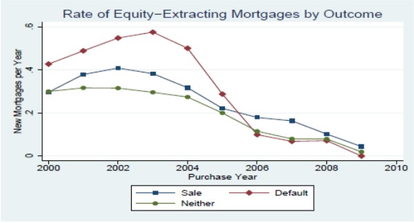
Examining this data set, I find that the impact of equity extraction on default differs depending on which cohort of home buyers we consider, with earlier purchasers having had more opportunity to extract equity during the boom. Figure 1 breaks down each quarter's defaulters from my Los Angeles data by the year of purchase. While most defaulters during the recent surge were owners who had purchased their homes within several years of the 2006 peak in house prices, a significant and increasing number of defaulters were from earlier cohorts of purchasers. By 2009, more than 40% of the homeowners defaulting each quarter had purchased their homes in 2003 or earlier. At the point where homeowners from this group defaulted, over 40% of their outstanding mortgage debt was attributable to equity extraction subsequent to purchase. The importance of equity withdrawals declines for later cohorts, becoming insignificant for buyers purchasing after the 2006 peak (See Figure 2). In this paper, I therefore focus on these earlier cohorts of buyers.

In Figure 3, I plot the distribution of estimated LTV ratios at the time of default for defaulting homeowners who purchased their homes between 2000 and 2003 and compare these LTV ratios to what they would have been had these homeowners not taken out additional mortgage debt.³ When these owners defaulted, I estimate that their average LTV ratio was just over 1.0, a quarter had LTV ratios over 1.4 and 10% had LTV ratios over 1.7. Without any equity extraction, the majority of these homeowners would have had LTV ratios under 0.6 and less than 10% would have had ratios that exceeded unity. Insofar as high LTV ratios were an important factor in these default outcomes, equity extraction is a key part of the story. There is also a significant difference in the rate of equity extraction between homeowners who ultimately defaulted and those who did not. In Figure 4, I compare the equity extraction rates of owners from each cohort who did and did not default during the observation period. Early buyers who remained in their homes throughout the sample period extracted equity at a rate of approximately once every three years. Among homeowners from this group who defaulted by 2009, the rate of equity extraction was 70% higher.⁴

Explaining this joint behavior of equity extraction and default decisions is made more difficult by limitations of the data. Many of the state variables that we expect to be important factors in these decisions, such as income, assets, the current house value, and expectations about future house prices, are all absent from my mortgage data, as they are from most other mortgage data sets. To fill in these gaps, I construct a dynamic model of homeowners who face both income and house price shocks and make decisions each period regarding savings, their mortgage balance, whether to sell their house and whether to default. The model is closest to those of Yao and Zhang (2008) and Campbell and Cocco (2011) with several important additions that allow me to capture important features of the data. First, in addition to permanent and transitory components, the income process includes a large discrete shock that I associate with unemployment and simulate to match evolving unemployment rates in the data. I find that these unemployment shocks are an important but not dominant driver of defaults. In the simulations, defaulters are five times more likely to be unemployed than the general population of homeowners but only 17% of defaulters are unemployed at the time of default.⁵Second, the model's treatment of house prices is novel in that it captures the predictability of short-term house price growth, as first documented by Case and Shiller (1989). Beyond the large movements in realized house prices, I find that changing expectations about future price growth is responsible for 20% of equity extraction when prices were rising during the boom and 34% of defaults as prices fell during the bust. Finally, I introduce a preference shock that accounts for the residual heterogeneity in the default decisions of underwater homeowners. This residual shock gives the model the flexibility to reproduce many of the patterns of household default decisions while maintaining income and house price shocks that are calibrated to match observable data.

I estimate the parameters of the model by matching a set of moments computed from the borrowing and default outcomes recorded in the CoreLogic mortgage data. In addition, the estimation draws on other data sources that contain information about the relationship between the model's unobserved states and observable information such as location, time period and features of the mortgages. I then use the estimated model to study the role of both income and house price shocks in homeowners' decisions to extract equity and default.

The model provides two key mechanisms that connect homeowners' equity extraction during the boom and their decision to default during the bust. First, homeowners who withdraw more equity end up with larger mortgage balances and larger mortgage payments, both of which directly increase the probability of default. Second, liquidity constrained households are more likely to extract equity in order to smooth consumption when hit by a negative income shock. This introduces a selection effect whereby those homeowners who take out larger mortgages are more likely to have fewer liquid assets and a history of negative income shocks, a condition that in itself increases the risk of default. Quantitatively, I find it is the direct effect of equity extraction rather than this selection effect that explains most of the connection between equity extraction and default. Income shocks and liquidity constraints account for only 30% of defaults following the decline in prices.

Using this estimated model, I study two counterfactual policies that would reduce homeowners' ability or incentive to extract equity. The first policy limits the amount of equity that existing homeowners can withdraw by prohibiting cash-out refinances from exceeding 80% of the current house value. This restriction is similar to a key provision of refinance policies currently in effect in Texas. In the second policy, I treat mortgages as full recourse loans. This means that after leaving the house, a defaulting borrower would continue to be obligated to repay the portion of the mortgage not covered by the sale price of the house. Most states allow the lender to take legal action against defaulting homeowners to enforce this obligation. California, however, where the present study is focused, is generally classified as a "non-recourse" states where such actions are prohibited.⁶

In the first policy experiment, I find that limiting the amount of equity that homeowners can extract reduces the amount of equity extracted during the boom by 23%. Because of the decreased collateral value of housing, prices fall by an average of 14% and the combination of lower house prices and less ability to borrow causes households to hold less debt and therefore to default at a lower rate. Of the homeowners who default in the baseline model, 41% do not under this policy. However, the overall default rate is only 28% lower. This is because of an offsetting increase in defaults that arises from the reduced borrowing opportunities for homeowners with small but positive amounts of equity. The inability of these homeowners to access this equity has two consequences. The first is to close a borrowing channel that could be used to prevent default should they experience a negative income shock and become liquidity constrained. The second effect is to reduce the value of staying in the home for homeowners with negative equity and the prospect of regaining some positive equity through price growth. By decreasing the value of having small levels of positive equity, this increases the probability that such households will default when presented with an opportunity to do so. The welfare gain of this restriction for new homeowners is equivalent to 3.2% of consumption due to the lower prices at which they can purchase housing. Under a more extreme version of the policy that prohibits homeowners from extracting any equity at all, the default rate falls to 20% of its original value. I therefore conclude that equity extraction was responsible for 80% of defaults among these early home-buyers, representing approximately 30% of the total number of defaults in Los Angeles County from 2006 to 2009.

In the other policy experiment, I find that granting full recourse to lenders reduces defaults significantly. First, because the mortgages that can be secured by the house are less valuable, house prices fall by 12% so homeowners have less expensive houses and smaller mortgages at the time of purchase. Second, because homeowners can no longer expect to be relieved of their repayment obligations upon default, they take on less debt, reducing their equity extraction during the boom by 18%. Finally, the policy creates a strong disincentive to default among homeowners who already have negative equity. The total default rate falls by 45%. I estimate that the overall welfare gain to new homeowners from this policy is equivalent to 2.7% of consumption, again due to the lower price of housing.

1.1 Related Literature

This paper contributes to several strands of the existing literature on default. Empirical studies of mortgage default such as by Deng, Quigley and Van Order (2000) and Bajari, Chu and Park (2008) have provided evidence for the importance of the LTV ratio in the default decision. This paper, in contrast, focuses on homeowners for whom the LTV ratio is endogenously determined so that quantifying the relationship between LTV ratios and defaults requires a model that also explains differences in borrowing decisions. Elul et al. (2009) further demonstrate the importance of the interaction between high LTV ratios and liquidity constraints in producing defaults. In the model presented in this paper, spending decisions made by households can cause them to exhaust their liquid assets so that the binding liquidity constraints also emerge as endogenous outcomes. Ghent and Kudlyak (2011) find that at a fixed level of negative equity, recourse decreases the probability of default by 30%. I argue that in addition to this effect, the threat of recourse results in homeowners approaching the default decision with less negative equity. On the subject of equity extraction, Hurst and Stafford (2004) show that homeowners with few liquid assets and a history of negative income shocks are more likely to extract equity. My model is consistent with their findings.

Regarding the relationship between refinancing and default, Foote, Gerardi and Willen (2008a) find that foreclosed homes in New England exhibited greater refinancing activity and tended to have more life-time mortgages than those that were not foreclosed upon. Mian and Sufi (2011) identify a correlation at the regional level between the rate of house price appreciation from 2002-2006 and the default rate between 2006-2008. Based on this relationship, they conclude that house price growth and the resulting equity withdrawal can account for 35% of the total number of defaults in this period. The conclusion supported by their analysis is that had prices not risen from 2002-2006, inducing homeowners to borrow against accumulated equity, the default rate during 2006-2008 might have been 35% lower. This differs from the counterfactual experiment that motivates the present study, in which house price growth is left unaltered but the borrowing opportunities of homeowners are changed.

Earlier structural models that include homeowners' mortgage choices and the option to default include Campbell and Cocco (2003), and Yao and Zhang (2008). More recently, Campbell and Cocco (2011) develop a model which focuses more on defaults but does not allow homeowners to refinance. An important difference between these papers and the present study is that I estimate my model using household-level data and am able to quantitatively match the cross-sectional and time series patterns of default found in that data. This provides me a realistic baseline model from which to run counter-factual policy experiments. Li, Lui and Yao (2008) also estimate a model of housing and mortgage choices using household data from the PSID, but in their model, homeowners never have an incentive to default.

A growing literature in macroeconomics studies the mortgage choices of homeowners in a general equilibrium setting in which prices are determined endogenously. Papers that study the effects of default risk on interest rates include Jeske, Krueger and Mittman (2010), Guler (2008), and Corbae and Quintin (2010). Chatterjee and Eyigungor (2009) study the equilibrium effects of default on house prices and include an analysis of the effects of foreclosure prevention policies on prices. Favilukis, Ludvigson, and Van Nieuwerburgh (2011) account for the boom and bust in U.S. aggregate house prices in a model where credit constraints on mortgages are relaxed and later re-tightened. The current paper does not attempt to solve for equilibrium interest rates. Also, while I do allow the overall level of house prices to adjust in response to policy changes, I the rate at which prices grow each period. This allows me to include a more realistic model of the income and house price risks that drive equity extraction and default.

The rest of the paper is organized as follows. In Section 2, I present a structural model of equity extraction and default. In Section 3, I describe my mortgage data set and the other sources of data on income and assets which I use to estimate the parameters of the model. I explain the estimation of this model in Section 4 and discuss the results of the estimation in Section 5. The policy experiments are described in Section 6. Finally, Section 7 concludes and discusses potential implications of my findings for current policy discussions.

2 Model

In this section, I describe a dynamic model of a homeowner who makes decisions about consumption and savings, is able to adjust his mortgage balance, and has the options to pay off his mortgage and sell the house or to default on the mortgage. The key novel feature is the set of shocks that allow the model to match the data: a large discrete unemployment shock, changing expectations about future house prices, and a continuous preference shock that captures residual heterogeneity in the default choices of underwater homeowners.

2.1 Preferences

Time in the model is discrete and households are infinitely lived. Each period, households consume housing services and non-housing consumption and receive utility

$\displaystyle u(c_t,h_t)=\frac{(c_t^\alpha h_t^{(1-\alpha)})^{(1-\gamma)}}{1-\gamma}.$

In addition to the quantity of housing and non-housing consumption, households have time-varying preferences each period over whether to remain in their current house or to move to a different house. I denote the utility derived each period from the decision over whether to stay or move by $\Omega_t$ with the details to be described below.

Preferences are time-separable with discount factor $\beta$ so that at time , households have preferences over

$\displaystyle \mathbf{E}_{t_0}\sum_{t=t_0}^\infty \beta^{(t-t_0)} (u(c_{t},h_{t}) + \Omega_{t})$

2.2 Income

Households have risky labor income that follows a process

$\displaystyle Y_t=P_t \varepsilon_t \;\;\;\;\;\;\; P_t= P_{t-1} \nu_t$

where

is the permanent component of income subject to shocks $\nu_t$ with $\log \nu_t \sim \mathcal{N}(\mu_\nu, \sigma_\nu^2)$ and $\varepsilon_t$ are transitory shocks. The transitory shock has two components, a discrete component $e_{t}$ corresponding to whether the household is unemployed for the period, and a continuous component $\varepsilon^0_{t}$ that captures all other transitory variation in household income. An unemployed household loses a fraction $(1-\delta)$ of its permanent income, so $e_t=\delta$ when the the household is unemployed and

otherwise. Employment follows a Markov process with constant transition probabilities into and out of unemployment given by $\pi_{e\rightarrow u}$ and $\pi_{u\rightarrow e}$ respectively. The continuous component $\varepsilon^0_{t}$ is i.i.d. and has a distribution $\log \varepsilon_t^0 \sim \mathcal{N}(0, \sigma_\varepsilon^2)$ . The total transitory shock is the product of the two components: $\varepsilon_{t}=e_t \cdot \varepsilon^0_{t}$ .

The discrete unemployment shock in the income process is not standard in this literature.⁷ I introduce it for two reasons. First, a large and persistent income shock is likely an important factor in a household's default decision. Second, the observed measure of income shocks present in the data is an estimate of the local unemployment rate. When I simulate the model, I draw realizations of this unemployment shock in a way that is consistent with the patterns of unemployment found in the data.⁸

2.3 Assets

Households hold three kinds of assets, a one-period bond, their house, and a mortgage. The bond earns a risk-free savings rate and must be held in positive quantity.

2.3.1 Housing

The household must hold an amount of the housing asset equal to the amount of housing services consumed that period, so both are identified with the quantity . The price per unit of housing is so the value of the house is . There is maintenance cost each period proportional to the value of the house, $\chi H_t$ . Households may sell their house and purchase a house of different size $h_{t+1} \neq h_t$ , also priced at , by paying a fixed cost $\theta_0 P_t$ and a transaction cost proportional to the value of the house being sold, $\theta_1 H_t$ . Finally, a household that moves to a different house incurs a utility penalty equal to

$\displaystyle \Theta_u=\theta_u P_t^{1-\gamma} p_t^{(1-\alpha)(\gamma-1)}$

The proportionality factor which multiplies $\theta_u$ maintains the size of this penalty relative to changes in income and price levels.⁹As I do not model the decision of the household to become an owner, I also assume that it does not consider the option of selling the house to become a renter.

Innovations to house prices have three components, two of which are common within the household's geographic region, indexed by , and one that that is idiosyncratic to the household. First, there is a persistent regional component $\mu_{jt}$ , which can take one of two values, $\mu_{jt} \in \{\mu_1,\mu_{2} \}$ and follows a Markov process with transition matrix $\Pi_{\mu,\mu^\prime}$ . Without loss of generality, I assume that $\mu_2>\mu_1$ so that $\mu_2$ represents the high-price-growth state. Second, there is an i.i.d. component to regional house prices $\eta_{jt} \sim \mathcal{N}(0,\sigma_\eta^2)$ . Finally, the is an i.i.d. idiosyncratic component $\zeta_{it} \sim \mathcal{N}(0,\sigma_\zeta^2)$ so that the total time- price appreciation of house in region is given by:

$\displaystyle \Delta p_{ijt}= \mu_{jt} + \eta_{jt} + \zeta_{it}.$

The expected price growth in the subsequent period,

$\displaystyle E_t \Delta p_{ij,t+1}= E(\mu_{j,t+1}\vert\mu_{jt}),$

is not constant over time, but depends on the current value of $\mu_{jt}$ .

I assume that households do not observe the true state $\mu_{jt}$ , but rather they observe a history of regional house prices { $\mu_{jt^\prime} + \eta_{jt^\prime}\}^t_{t^\prime=-\infty}$ and solve a filtering problem to determine the probability distribution $f_{jt}(\mu)$ over the two states $\{\mu_1,\mu_{2} \}$ in each period.¹⁰ This distribution, which can be summarized by $f_{jt}(\mu_2)$ , the probability that region is in the high-appreciation state at time , becomes a state variable in the household problem.¹¹

2.3.2 Mortgages

The household holds a mortgage of size on which it makes interest payments but does not pay down the principal.¹² Homeowners may change the size of their mortgage, subject to two restrictions on the new mortgage. The first restriction is that the new total mortgage balance may not exceed a fraction $\phi_{jt}$ of the current house value. This limit on the LTV ratio may depend on current beliefs about future house prices, so that lending standards are looser if prices are expected to rise, i.e. $\phi_{jt}=\phi(f_{jt}(\mu_2))$ , where the function $\phi(\cdot)$ is increasing. There is no period-by period borrowing constraint so the LTV ratio, , may become arbitrarily high if house prices decline. The second restriction is that mortgage payments may not exceed a fraction $\psi_i$ of permanent income, $r^m M_{t+1}< \psi_i P_t$ , where $i \in \{P,R\}$ depending on whether the mortgage is for a new purchase (P) or to refinance the mortgage on the current home (R).

There are two costs associated with refinancing a mortgage, a fixed cost, which is fraction of permanent income, and a fraction of the the total size of the new mortgage. Although the interest rate on all allowed mortgages is the same, households wishing to borrow an amount greater than $\overline{m}$ of the house value pay an additional one-time cost $k_2M_{t+1}$ . This additional cost captures actual costs such as mortgage insurance, as well as higher interest rates paid by borrowers taking out riskier mortgages.¹³ There is no cost associated with paying off the current mortgage and not taking out a new one. Thus the total cost of choosing a new mortgage $M_{t+1} \neq M_t$ with $M_{t+1}>0$ is $K(M_{t+1})=k_0P_t +(k_1+k_2 \cdot \mathbf{1}(M_{t+1}>\overline{m}H_t))M_{t+1}$ .

When the house is sold, the balance of the mortgage is repaid from the proceeds of the sale. If $M_t>(1-\theta_1)p_th_t$ , then the funds generated by the sale are insufficient to repay the mortgage debt. In the data, I do see sales occurring for houses that appear to be worth less than the outstanding mortgage balance. To capture this feature of the data, I allow homeowners to repay the balance of the mortgage in excess of $(1-\theta_1)p_th_t$ out of savings. However, to do so, they incur a cost $\kappa \cdot (M_t-(1-\theta_1)p_th_t)$ , which is proportional to the amount of mortgage debt being repaid from sources other than sale of the home. If $\kappa=0$ , then homeowners freely pay off excess mortgage debt from their liquid assets. As $\kappa \rightarrow \infty$ , households are unable (or unwilling) to use funds from other sources in order to pay off the mortgage. In reality, there is little evidence that homeowners contribute other funds towards the repayment of a mortgage balance that is not covered by the sale price of the house. Rather, a finite value of $\kappa$ likely describes the willingness of banks to engage in short sales and to release the lien and accept the sale price as repayment even if it falls short of the outstanding debt. However, I do not model such short sales explicitly.¹⁴

2.4 Default

Mortgage default is modeled in a way to capture the fact that loans in California are non-recourse. Homeowners defaulting on their mortgages remain in their houses for the current period but do not have to make mortgage or maintenance payments. At the end of the period, they pay moving costs $\theta_0 P_t$ (but not the transaction cost $\theta_1 H_t$ ) and retain any remaining liquid assets $a_{t+1}$ . They incur the non-monetary moving cost $\Theta_u$ and permanently enter a frictionless rental market in which housing services are available at price $\rho p_t$ . A household that cannot afford its mortgage and maintenance payments and does not have feasible options among changing its mortgage position or house size is forced to default. A household that does have other feasible options may still choose to default as an optimal decision.

2.5 Preference Shocks

Every period, the household receives a preference shock of strength $\omega_t$ that controls its preference for remaining in the current house. If the household leaves its house during this period, either by selling or defaulting, it receives additional utility

$\displaystyle \Omega_t=\omega_t P_t^{1-\gamma} p_t^{(1-\alpha)(\gamma-1)}.$

With probability $\lambda$ , the "strength" of the preference shock $\omega_t$ is non-zero and follows an i.i.d. distribution $\omega_{t} \sim \mathcal{N}(\mu_\omega,\sigma_\omega^2)$ . With probability $(1-\lambda)$ , there is no shock and $\omega_t=0$ . The proportionality factor between the strength of the shock $\omega_t$ and the total utility $\Omega_t$ is the same one used for $\Theta_u$ , the dis-utility of moving.

This preference shock generalizes the "moving shock" that Cocco (2005) and others have introduced in order to match the rate at which homeowners sell their homes. In the limit $\mu_\omega \rightarrow \infty$ , homeowners always move in response to this shock and it becomes equivalent to the moving shock of previous models. Allowing this shock to arrive with different strengths provides a range of realizations for which homeowners whose mortgage balances far exceed their house values will default but those with mortgages only slightly above their hose house values will remain in their homes. This allows me to better match the increasing rate of default among homeowners with higher amounts of negative equity.

2.6 Household Problem

The problem faced by the homeowner each period can be written recursively. The solution to this problem is given by a value function

$\displaystyle V(P,\tilde{a},h,e,p,M,\Omega,f)$

where

is permanent income, $\tilde{a}=a+P\varepsilon$ is cash-on hand,

is the size of the house,

indicates if the homeowner is employed, the price of housing is given by

so that the value of the house is

is the mortgage balance, $\Omega$ is the current realization of the preference shock and $f=f(\mu_2)$ is the filtered probability of being in the high-price-growth state. The household then has a choice over the following four options with regard to housing and mortgages, each with an associated value function. In each option, the household also chooses non-housing consumption

.¹⁵

Continue to pay the mortgage

$\displaystyle V^0(P,\tilde{a},h,e,p,M,\Omega,f)=\max_{c} u(c,h)+\beta \mathbf{E}V(P^\prime,\tilde{a}^\prime,h,e^\prime,p^\prime,M,\Omega^\prime,f^\prime)$

$\displaystyle a^\prime=(1+r^s)\cdot(\tilde{a} -\chi ph-r^mM -c), \;\;\; a^\prime \geq 0$
Refinance into a new mortgage of size $M^\prime \neq M$ . The amount of equity extracted is equal to $(M^\prime-M)$

$\displaystyle V^R(P,\tilde{a},h,e,p,M,\Omega,f)=\max_{c,M^\prime} u(c,h)+\beta \mathbf{E}V(P^\prime,\tilde{a}^\prime,e^\prime,h,p^\prime,M^\prime,\Omega^\prime,f^\prime)$

$\displaystyle a^\prime=(1+r^s) \cdot(\tilde{a}+(M^\prime-M)-r^m M-\chi ph -K(M^\prime)-c), \;\;\; a^\prime \geq 0, \;\;\; M^\prime<\phi(f)ph, \;\;\; r^m M_{t+1}< \psi_R P$
Sell the house and purchase a new house of size $h^\prime$ with a new mortgage $M^\prime$

$\displaystyle V^S(P,\tilde{a},h,e,p,M,\Omega,f)=\max_{c,h^\prime,M^\prime} u(c,h)+\Omega - \Theta_u +\beta \mathbf{E}V( P^\prime,\tilde{a}^\prime,e^\prime,h^\prime,p^\prime,M^\prime,\Omega^\prime,f^\prime)$

$\displaystyle a^\prime=(1+r^s) \cdot (\tilde{a}+(1-\theta_1-\chi)ph-\theta_0P-(1+r^m)M-ph^\prime+M^\prime$

$\displaystyle \;\;\;\;\;\;\;\;\;\;\;\;\;\;\;\;\;\;\;\;\;\;\;\;\;\;\;\;\;\;\;\;\;\;\;\;\; -\kappa(M-(1-\theta_1)ph)\cdot \mathbf{1}((1-\theta_1)ph<M)-c)$

$\displaystyle a^\prime \geq 0,\;\;\; M^\prime<\phi(f)ph^\prime, \;\;\; r^m M_{t+1}< \psi_P P$
Default

$\displaystyle V^D(P,\tilde{a},h,e,p,M,\Omega,f)=\max_{c} u(c,h)+\Omega - \Theta_u +\beta \mathbf{E}V^{rent}(P^\prime,\tilde{a}^\prime,e^\prime,p^\prime)$

$\displaystyle a^\prime=(1+r^s) \cdot (\tilde{a} -c -\theta_0P), \;\;\; a^\prime \geq 0,$

where $V^{rent}$ solves the renter's problem, defined below.

Expectations are taken over the possible realizations of the permanent and transitory income shocks, the unemployment shock, the regional and idiosyncratic house price shocks and the preference shock.¹⁶ The value function is the maximum value of these four choices

$\displaystyle V(P,\tilde{a},h,e,p,M,\Omega,f)=\max(V^0(\cdot),V^R(\cdot),V^S(\cdot),V^D(\cdot)).$

After default, renters make decisions over the housing and non-housing consumption. Renters are not responsible for maintenance costs and can costlessly adjust their housing consumption. The renter's problem can be written

$\displaystyle V^{rent}(P,\tilde{a},e,p)=\max_{c,h} u(c,h)+\beta \mathbf{E}V^{rent}(P^\prime,\tilde{a}^\prime,e^\prime,p^\prime)$

$\displaystyle a^\prime=(1+r^s) \cdot (\tilde{a} -c -\rho ph), \;\;\; a^\prime \geq 0.$

2.7 Model Solution

The model has been constructed so that it is possible to reduce the dimension of the state space by rewriting the problem in terms of variables that are normalized by permanent income: $\hat{a}=\tilde{a}/P, \hat{H}=H/P,$ and $\hat{m}=M/H$ .¹⁷ In this formulation, neither the level of permanent income , nor the level of housing prices enters the household problem explicitly, greatly reducing the size of the state space and the computational burden of solving the model. Details are shown in an appendix.

Once the problem has been expressed in these normalized variables, I discretize the state space and the control space and then solve the household problem using value function iteration. At values in between these discrete points, I approximate the value function using linear interpolation.

3 Data

In this section, I describe the sources of data that I use to estimate the parameters of the model presented above.

3.1 Liens Data

The main data set used in this analysis is a series of quarterly "open lien searches" conducted by CoreLogic on all single family residences in Los Angeles County, California from 2000 to 2009.¹⁸ These searches identify all outstanding mortgages currently open against each property. As described in the introduction, the novel feature of this data set is that the unit of analysis is the property rather than the mortgage. Because it is possible to link together all the mortgages taken out against each property, I can compute the total mortgage balance and measure equity extraction.

At the start of 2000, the data contains 1.2 million properties. As new residences are built, the number rises, reaching 1.3 million by the end of the sample. Each property is identified by unique numerical identifier as well as the postal address, which I use to identify the 2000 census tract and other geographical information. For each quarterly observation, the data include information about the most recent sale, including the date, the purchase price, a calculation of the combined LTV ratio at purchase, and whether it was a foreclosure sale. Including multiple owners of the same property, the data contains 1.9 million distinct ownership episodes.

3.1.1 Mortgages

In each quarter, the data includes information on up to four mortgages held against the property. For each mortgage, the data identifies the date and original amount of the loan, the maturity date, whether it was a purchase, refinance or junior mortgage, and the type of mortgage (conventional, FHA, VA etc.) There is additional information on junior mortgages such as whether it is a second or revolving mortgage. For most mortgages, the data also includes the interest rate and whether that rate is fixed or adjustable.¹⁹ A subset of adjustable rate mortgages, mostly from the end of the sample, also includes detailed information on the the contractual details governing rate adjustments.

There is no information about FICO scores or whether the loan is prime or sub-prime, but for many mortgages, there is an indicator of whether the mortgage lender is identified as a lender specializing in sub-prime mortgages. Gerardi et al. (2007) show that this measure is highly correlated with whether the loan itself can be categorized as sub-prime. Of the houses purchased after the start of the sample period, this indicator is present for 79% of purchase mortgages in the sample, with 22% of those mortgages classified as sub-prime. As shown in Table 1, the fraction of homes purchased with mortgages from sub-prime lenders grows from 14% in 2001 to 28% in 2004-2005 and drops off dramatically after 2006.

Although the data does not include payment history, CoreLogic calculates the outstanding balance on each mortgage each quarter using a proprietary algorithm. This allows identification of which refinances involve the extraction of equity. Figure 5 shows the number and type of new mortgages taken out each quarter, dividing these mortgages into cash-out refinances, non-cash-out refinances and junior mortgages. The rate at which new mortgages are taken out grows by a factor of five from 2000 to 2003, driven largely by cash-out refinances, and by a surge of non-cash-out refinances as interest rates reached historically low levels in 2003. From 2004 to 2007, approximately one in 12 homeowners took out an additional mortgage or withdrew cash through refinancing each quarter. The rate of cash-out refinancing falls as housing prices begin to decline in 2007, reaching a low point at the height of the financial crisis in 2008 before rebounding slightly in 2009.

3.1.2 Default

The data does not include information about whether a borrower has become delinquent. However, if the bank files a notice of default, which it must do to begin the foreclosure process, or a notice of trustee sale, indicating that it has set a date to sell the property, the types and dates of such filings are recorded in the data. The first filing of either of these notices is my measure of mortgage default. Although the notice of default can be filed up to one year after the borrower becomes delinquent, common practice in California is to issue such a notice when the mortgage becomes 90 days delinquent.

In Figure 1, I plot the total number of homeowners defaulting on their mortgages each quarter, broken down by the year of purchase. The default rate starts rising dramatically in 2006 when local house prices stop rising and begin to fall. By 2009, over 12,000 borrowers (more than 1% of all homeowners) are defaulting each quarter. Though these borrowers are disproportionately owners who purchased after 2003, a significant and increasing number of defaulters are drawn from earlier cohorts of purchasers. As I described in the introduction, only for these earlier homeowners did equity extraction play an important role in determining whether they later defaulted.

In Figure 6, I show the fraction of each cohort of buyers who are observed to sell or default by the end of the sample. Of the buyers who purchase in 2006, 40% have already defaulted by the end of 2009. The default rate is far lower for earlier cohorts, with only 7-8% of buyers from 2000-2002 having defaulted by the end of the sample period.

3.1.3 House Prices and Loan-to-Value Ratios

The borrower's combined LTV (cLTV) ratio is a key state variable in the model. The cLTV ratio at the time of purchase is included in the data. Table 1 shows that the mean cLTV ratio at purchase is 0.86-0.87 for most of the sample, rises to 0.88 in 2005 and then jumps to .90 in 2006 before falling down to 0.85 in 2007. The median cLTV ratio shows a similar behavior. A more striking pattern can be seen by looking at the fraction of purchases each quarter that were financed with mortgages with a cLTV ratio greater than or equal to 1.0. I plot this measure in Figure 7. The fraction rises from 10% to over 50% in the last quarter of 2006 and then declines precipitously to less than 2% by the middle of 2008.²⁰

In subsequent periods, computing the LTV ratio²¹ requires first having an estimate of the current house value. To estimate the house value in each period, I first compute a local zip-code-level house price index. I then construct an estimate of the value of each house each quarter by starting with the observed purchase price and assuming that the rate of appreciation each quarter is equal to the growth in the local price index. By combining this value estimate with the total outstanding mortgage balance, I can construct an estimate of the LTV ratio for each observation.²²

To calculate the house price index, I use the purchase information in the liens data to identify properties for which I observe multiple sales. I use these sales to construct a zip-code level repeat-sales housing price index, following the modification of Deng, Quigley and Van Order (2000) to the original algorithm of Case and Shiller. I perform kernel-weighted local polynomial smoothing across time on the resulting quarterly price estimates. Properties in the data are spread over 302 zip codes, and there are a sufficient number of transactions to generate reasonable house price series for approximately 250 of these zip-codes for the period 1986-2009. Though there is substantial variation in the size of the price fluctuations, most zip-codes exhibit similar trends, a peak in house prices around 1990, followed by a moderate decline and then a rapid appreciation starting around 2000. Prices peak in 2006 before declining dramatically and then appear to level off or even slightly recover in the final quarters of 2009. Average price increases from 2000 to 2006 were approximately 150% followed by a decline of almost 50%. A sample of house price indices for several zip-codes is shown in Figure 8.

3.1.4 Estimation Sample

I focus the analysis on earlier cohorts for whom equity extraction was an important factor in determining if they ultimately defaulted. For my estimation, I select houses purchased in 2002-2004. I exclude owners who have purchased their house through a foreclosure sale, houses that are not owner-occupied, and those with missing or outlying values of any variables used in the analysis. I further exclude homeowners with government loans insured by the Federal Housing Administration or guaranteed by the Veterans' Administration, mortgages with terms less than 15 year or greater than 40 years, those houses in zip-codes with fewer than 1000 observed repeated house sales, and houses that do not appear in the data in the quarter in which they were purchased. Of the 100,000 houses meeting these criteria, I randomly select 20% to keep the computations manageable. I include observations from the time of purchase through the second quarter of 2009.

The resulting sample contains 20,531 homeowners across 1,691 census tracts and 230 zip-codes. The median purchase price is $375,000 with a mean of $462,000 and a standard deviation of $341,000. Twenty-seven percent of the sample borrowed their purchase mortgages from a sub-prime lender. Fifty percent took out a second mortgage at the time of purchase and the combined LTV ratio at purchase has a mean of .875, a median of 0.9 and it is greater than or equal to unity for 26.2% of purchasers.²³ The 42.7% of homeowners who purchased their homes with a fixed-rate mortgage have an average interest rate of 6.2%, with a standard deviation of 0.5%. Homeowners with adjustable-rate mortgages have an average interest rate of 5.9% with a standard deviation of 1.1%. The average household in this sample takes out 2.5 new mortgages during the sample period. Of these, 10% are non-cash-out refinances, 45% are cash-out refinances, 10% are home equity lines of credit and another 22% are classified as equity mortgages. By the end of the sample, 11% have defaulted and 27% have sold their homes without defaulting.

3.2 American Community Survey

Though I do not have observations of income shocks for individual households, I compute measures of local income shocks from the American Community Survey (ACS), an annual survey conducted by the U.S. Census Bureau since 2001.²⁴Unemployment rates can be computed from this data for each congressional district, broken down by race and age group.²⁵ I use software purchased from Geolytics to identify the congressional district of each property in the liens data, which spans 17 districts. Within each congressional district, I compute a local unemployment rate as a weighted average of the age-race specific rates. For weights, I use the demographic distribution of homeowners in the property's census tract from the 2000 census, also identified using the Geolytics software. When averaged across the sample, this rate begins below 5% in 2002-2003 and reaches 9.2% in 2009 during the recession.

The ACS also reports median annual household income among homeowners for each congressional district. I use growth in this statistic as an additional measure of local income shocks. The average growth rate fluctuates between three and five percent over most of this period but becomes negative in the final year of the sample.

3.3 Panel Study of Income Dynamics

The mortgage data includes no information about income or assets. Instead, I impute starting income and asset values for these homeowners by using observations of new homeowners in the Panel Study of Income Dynamics (PSID). The PSID is a longitudinal household survey conducted by the University of Michigan that has followed approximately 5000 families since 1968. The survey has been conducted biannually since 1997 and each wave since 1999 contains self-reported house values, a detailed breakdown of household income and asset holdings, and information about mortgages, including the principal balances, monthly payments, and interest rates. In particular, I am interested in the empirical relationship between assets and income and household characteristics present in my mortgage data set, such as initial LTV ratios and interest rate types and spreads.

I construct a sample of homeowners from the 1999-2007 waves who report having moved into their current residences within the 12 months preceding the interview and have a mortgage. For each household, I calculate two variables: the ratio of their after-tax household income to their mortgage payments and the total amount of liquid assets.²⁶ The logarithm of the ratio of income to mortgage payments is well approximated by a normal distribution with mean of 1.4 (an absolute value of 4.1) and a standard deviation of 0.6. The median value of liquid assets is is $5000 and the 75th percentile is $20,000. Ten percent of new homeowners report no liquid assets.

I regress the logarithm of both variables on a set of covariates that can be computed from both the PSID and the liens data set: the combined LTV at purchase, whether there was a second mortgage at the time of purchase, a dummy for whether the purchase mortgage had an adjustable interest rate, a measure of the interest rate spread,²⁷ and a dummy for whether the purchase occurred after 2005. Summary statistics for these covariates are shown in Table 2 and the results of these regressions are presented in Table 3. The regression of the ratio of income to mortgage payments uses 782 observations. Home buyers with higher LTV ratios have higher mortgage payments relative to their incomes. The 12% of buyers who purchase their homes using more than one mortgage have payments that are 20% higher than those without a second mortgage, and those buying after 2005 have higher payments by 13%. None of the other coefficients are significant. For assets, I estimate a Tobit model on 706 households with left-censoring at $1000. Those who purchase houses with a higher combined LTV have significantly fewer assets, as do those paying higher interest rates. Each additional percent on the interest rate corresponds to a decrease in assets of 38% for those with fixed-rate mortgages and 52% for borrowers with adjustable-rate mortgages.

The PSID also contains panel data on household income, which I use to calibrate the income process of the structural model presented above. I use the data set of after-tax household income constructed by Heathcote, Perri and Violante (2010), keeping only recent observations (after 1980) and only observations of homeowners, so as to better match my sample of post-2000 homeowners. This leaves me with 33,725 observations in which I can measure the growth of household income from one year to the next. I describe the calibration of the income process based on this data when I discus the parameterization of the model below.

3.4 Empirical Results

Before describing the estimation of the full structural model, I first estimate an empirical model of sales, equity extraction and default to study the dependence of these outcomes on observable household and local characteristics. I use the same estimation sample described above, dropping 355 observations with outlying values of some variables used in the estimation. I follow each house from purchase through the second quarter of 2009, creating a panel of 311,367 household-quarter observations of 20,176 distinct households. As I follow my estimation sample across time, I observe regional income shocks. My measure of the unemployment rate averages 5.7% with a standard deviation of 1.7%. Annual changes in median income levels average 4.0% with a standard deviation of 6.6%. Local house prices are recorded at the zip-code level. The sample spans 230 zip codes. One year house price appreciation averages 6.4% with a large standard deviation (17.0%) that captures a tremendous price increase through 2006 followed by a steep decline.

In each quarter, I consider four possible outcomes,

The owner chooses to extract equity, either through a cash-out refinance or an additional junior mortgage.
The owner sells the house and pays off the mortgage.
The owner defaults on the mortgage, which I see in the data when the bank issues a notice of default.
The owner makes none of the above choices, either continuing to pay all mortgages or refinancing without withdrawing equity.

I estimate a multinomial logistic regression with these four possible choices, with the last option, continuing to make payments, as the reference category. The estimation includes a set of fixed effects for the year of observation interacted with the year of purchase. Table 4 gives definitions and summary statistics for the variables used in the regression. Results are shown in Table 5.

High cumulative loan-to-value ratios at purchase, high interest rates, having an adjustable rate mortgage, and borrowing from lenders specializing in sub-prime mortgages are all associated with a greater propensity both to extract equity and to default. Comparisons to other data sets, such as the PSID, that include both mortgage information and other asset holdings suggest that high LTV ratios and high interest rates at purchase are both associated with low holdings of liquid assets. Households with LTV ratios above unity are more likely to default and this risk increases somewhat with higher LTV ratios. As the LTV ratios increases above one, households are also less likely to extract equity as there is no longer any equity to withdraw. High price growth leads to greater equity extraction, while negative house price appreciation is associated with higher default rates. Higher local unemployment rates are also associated with a greater likelihood of defaulting. Turning to local demographics from the 2000 census, I find that in locations with more educated populations, homeowners are somewhat more likely to take advantage of opportunities to extract equity and also somewhat less likely to default. These findings are consistent with a large body of previous work.

With regard to selling one's house, I find that households in areas with more homeowners under age 35 are more likely to sell, as are home buyers who purchase their homes with an adjustable rate mortgage, a high-LTV mortgage, or a mortgage with a higher interest rate. These latter measures are probably also indicative of younger owners with lower accumulations of liquid savings. Positive house price growth also increases the probability of sale as it give homeowners the positive equity they need to be able to sell.

I next attempt to match the moments from this estimation using the full structural model presented above.

4 Model Estimation

I estimate the key parameters of the model using the simulated method of moments. Several parameters, however, such as the processes for household income and house prices, rely on other data and are estimated separately.

A period in the model corresponds to one quarter. All quantities in the model are nominal.

4.1 Income

The income process has three components: the permanent shock, the discrete unemployment state, and the continuous transitory shock. I calibrate each of these outside the estimation.

The probability that an employed worker will become unemployed, $\pi_{e\rightarrow u}$ is an important parameter in matching the default rate and I estimate it jointly with the other parameters of the model, as described below. Conditional on its value, I fix the transition rate out of unemployment $\pi_{u\rightarrow e}$ to achieve a steady state level of unemployment consistent with the data. The average unemployment rate in my sample is 6.2%. However, this rate combines both homeowners and non-homeowners, while I am interested only in the rate among homeowners. In order to estimate the difference in unemployment rate by homeownership status, I use PSID data to estimate a logistic regression of the unemployment status of the head of household on homeownership status, also including dummies for race and a quartic polynomial in the age of the head. I estimate an odds ratio of 0.31 for homeownership, meaning that controlling for age and race, a homeowner is only 31% as likely as a renter to be unemployed. Assuming the total population contains 63% homeowners, which is the average census-tract-level homeownership rate in my sample from the 2000 census, this implies that the unemployment rate among homeowners is 55% of the overall rate. Therefore I target a steady-state unemployment rate of $0.55 \times 6.2\% = 3.4\%.$ I estimate a value $\pi_{e\rightarrow u}=0.020$ , which implies a job finding probability $\pi_{u\rightarrow e}$ =0.60, implying a median unemployment spell of just under one quarter. The average wage replacement rate in California is 50% so I set the replacement rate $\delta=.5$ .

Following Heathcote, Perri and Violante (2010), I calibrate the remaining parameters of the income process to match the mean, the variance and the one-period auto-covariance of the one-year growth in household after-tax log income, using only recent observations of homeowners in their data.²⁸ Given my estimates for the unemployment process, the resulting parameters are $\mu_\nu=.008, \sigma_\nu=.096$ for the permanent shock and $\sigma_\varepsilon= .233$ for the transitory one.

4.2 House Prices

To estimate the parameters of the house-price process, I use properties from the liens data with multiple recorded sales after 1986 to construct quarterly, zip-code-level repeat-sales house price indices using the algorithm from Deng, Quigley and Van Order (2000). The long-run growth rate of housing prices is poorly identified from this window, which contains approximately two full cycles of price growth and decline. When I estimate the model of regional house prices using these zip-code-level indices, I impose the additional constraint that the annual nominal long run growth rate in house prices equal 4%. I estimate mean appreciation in the two regimes to be $\mu_1=-.018, \mu_2=0.038$ with transition probabilities $\Pi_{1,2}=.092, \Pi_{2,1}=.046$ and a standard deviation of the regional i.i.d. house shock $\sigma_{\eta}=.02.$ This means that during a boom, homeowners expect prices to grow at 3.8% quarterly and for this appreciation to continue on average for 22 quarters. In periods of declining house prices, average declines are 1.8% per quarter and last for 11 quarters on average.

In addition to changes in regional house prices, households face quarterly idiosyncratic price shocks $\zeta_{it} \sim \mathcal{N}(0,\sigma_\zeta^2)$ . Consider a house in region that sells in period $\tau$ at price $p_{i\tau}$ and then again in period $\tau^\prime$ at price $p_{i\tau^\prime}$ . If the zip-code level house prices indices at the times of the two sales are $p_{j\tau}$ and $p_{j\tau^\prime}$ , then the idiosyncratic portion of the change in prices

$\displaystyle (p_{i\tau^\prime}-p_{i\tau})-(p_{j\tau^\prime}-p_{j\tau})=\sum_{\tau+1}^{\tau^\prime} \zeta_{it}$

is distributed $\mathcal{N}(0,(\tau^\prime-\tau)\sigma_\zeta^2)$ and I can identify $\sigma_\zeta^2$ as the sample variance of

$\displaystyle \frac{(p_{i\tau^\prime}-p_{i\tau})-(p_{j\tau^\prime}-p_{j\tau})}{(\tau^\prime-\tau)}.$

Depending on how I choose the the sample of repeat sales for this estimation, I get values of $\sigma_\zeta$ between .015 and .019. I choose the middle of this range, $\sigma_\zeta=.017$ .

In the data, I observe a correlation of 0.17 between the growth rates of median income and the zip-code-level house price index. However, there is also a significant amount of additional idiosyncratic variation in both income and house price growth for individual households. Using the calibrated parameters of my income and house price processes, I estimate that the correlation between house prices and permanent income for an individual homeowner is only 0.03.²⁹ This is the value I use in the model.

4.3 Other Parameters

I fix the quarterly return on savings at and the mortgage interest rate at , the average interest rate in my sample. Quarterly maintenance costs are fixed at a fraction $\chi=.003$ of the house price, consistent with spending on alterations and repairs reported by respondents in the American Housing Survey.³⁰ During the boom, it was common to take out a mortgage equal to 100% of one's house value so I set the limit on LTV ratios for new mortgages during periods of positive expected price growth to $\phi(f(\mu_2)=1)=1.0$ . After the crash, lending standards tightened and I use an 80% limit for periods of negative expected price growth, $\phi(f(\mu_2)=0)=0.8$ . At intermediate values, I assume the limit is piecewise linear and include the value of $\phi(f(\mu_2)=0.5)$ in the list of estimated parameters. Finally, I impose the additional borrowing costs for riskier mortgages on mortgages that exceed a threshold fraction $\overline{m}=0.8$ of the value of the home. This is the LTV ratio above which private mortgage insurance is typically required.

4.4 Simulations

This leaves 18 model parameters that are key for matching patterns of sales, equity extraction and default found in the data: the three preference parameters $\beta,\gamma, \alpha$ , borrowing limits $\psi_P$ , $\psi_R$ and $\phi(f(\mu_2)=0.5)$ , mortgage costs $k_0,k_1,k_2, \kappa$ , moving costs $\theta_0,\theta_1,\theta_u$ , the rent-price ratio for defaulters $\rho$ , parameters of the preference shocks $\lambda, \mu_\omega,\sigma_\omega$ and the rate of job loss $\pi_{e\rightarrow u}$ . These parameters are estimated using the simulated method of moments.

Each of the 20,531 households in my estimation sample is simulated 25 times. Simulations begin at the time of purchase and end when the homeowner moves or defaults, or reaches the end of the sample period, which extends to second quarter of 2009. This creates a maximum sample period of 30 quarters. The probability that an employed homeowner loses his job is held constant at $\pi_{u\rightarrow e}$ and I vary the probability with which an unemployed worker becomes employed to reproduce the current local unemployment rate.³¹ Shocks to permanent income are drawn from a normal distribution with a mean to match the period and region specific growth rate of median income.

The evolution of regional house prices follows the observed zip-code level house price indices calculated from the data. For each period, in each zip-code, I update $f(\mu_2)$ using the same filtering algorithm attributed to agents in the model. In Figure 9, I plot the distribution of $f(\mu_2)$ across zip-codes at different times. This graph shows that until mid-2005, all households expected prices to continue rising. By the end of the boom in mid-2006, approximately half of households still believed that the probability of continued price growth was greater than 50%. The model predicts that by the start of 2008, all homeowners in the sample would have believed that prices would continue to fall.

The continuous transitory income shocks and idiosyncratic house price shocks are drawn from their unconditional distributions.

I match a set of 190 observable moments motivated by the empirical analysis of the Section 3.4. These moments include the rates of new mortgage origination (excluding non-cash-out refinances), default and sale each quarter, plus the interaction of these rates with unemployment, median income growth, house price appreciation, LTV ratio at purchase and the current observed LTV ratio. I also target the rates of default and sale by LTV ratio, the LTV ratio of homeowners each period who do and do not default, the total number of households who sell and default, and the rate of equity extraction by purchase year and outcome. From the PSID data on new homeowners, I target the average value of mortgage payments as a fraction of income and the the 50th and 75th percentiles of the distribution of liquid assets.³²

Due to the computational demands of this estimation, I use a parallelized implementation of the Nelder-Mead simplex algorithm, as described in Lee and Wiswall (2007).³³

4.4.1 Initial Conditions

Each simulated household begins with a level of permanent income and an endowment of liquid assets, already having decided to purchase a house and now optimizing over the size of that house and a starting mortgage balance. Equivalently, the household makes choices over the starting LTV ratio and the fraction of its income consumed by its mortgage payments. The procedure by which I assign these starting values for income and assets is designed to satisfy two objectives. First, the model makes predictions about the optimal choice of house size and mortgage balance for each starting value of income and assets. Starting values should be assigned so that, on average, household are making choices consistent with these predictions. Second, based on my analysis of new homeowners in the PSID, there is significant heterogeneity in assets and income of homeowners immediately after purchase. Most of this heterogeneity cannot be explained based on observable characteristics of the household. However, analysis of these new homeowners reveals that there are statistically significant correlations between starting income and assets and some characteristics that are observable in the data. Most notably, homeowners with higher interest rates tend to begin with lower asset holdings but do not have larger mortgage payments relative to their income. (See Section 3.3.) These correlations should be reproduced in the simulations. The procedure by which I assign the initial conditions satisfies these two objectives. Details are described in an appendix. This procedure defines three additional free parameters, which I estimate jointly with the other parameters of the model. The definitions and estimated values of these parameters are contained in the appendix. Finally, I assume that homeowners are employed at the time of purchase.

5 Estimation Results

5.1 Parameter Estimates

Parameter estimates are are shown in Table 6. I find a quarterly discount factor of 0.94. This low value is consistent with the fact that households only extract equity when they deplete their liquid assets and in the data, new equity-extracting mortgages are initiated every 10-12 quarters. In the model, all spending beyond mortgage and maintenance payments is attributed to consumption and so the rapid rate at which assets are exhausted means that the desire for immediate consumption is very high and the discount factor must be low.³⁴ The estimate of risk aversion is $\gamma=1.52.$ The share of housing consumption in the utility function is $(1-\alpha)=.26$ , slightly higher than, for example, the 19% share of 2005 expenditures spent on shelter according to the Consumer Expenditure Survey, and consistent with the fact that housing costs in Los Angeles are higher than the national average. The estimated values of mortgage costs and mean that the cost of new mortgages is 15% of quarterly income income, which is approximately ten days worth of earnings, plus 1.2% of the value of the mortgage. This is slightly higher than actual initial mortgage fees, which averaged approximately 0.5% during this period according to the Federal Housing Financing Board's Monthly Interest Rate Survey.

Homeowners wishing to take out loans with LTV greater than 0.8 must pay a fraction of the entire balance. This can be thought of as approximately seven to ten years of mortgage insurance payments, which are typically just under one percent of the total loan balance per year.

New buyers are restricted from taking out mortgages whose payments are greater than $\psi_p=38\%$ of their after-tax income. For the sake of comparison, guidelines for conforming conventional loans call for mortgage payments not to exceed 28% of the borrower's gross income. I estimate that there are no income limits on homeowners wishing to refinance, i.e. a value of $\psi_r$ sufficiently large that it is a non-binding constraint. This estimate is necessary for the model to reproduce the higher rate of equity extraction among defaulters compared to non-defaulters. Homeowners who ultimately defaulted tended to already have larger mortgages at the time of purchase, but this group of homeowners nevertheless extracted equity at a greater rate than those who did not default. This suggests that households who already had significant mortgage obligations were committing increasingly large fractions of their income to debt payments as prices climbed. Overall, the median household in my estimation sample increases its mortgage balance by 20% and a quarter of homeowners expand their debt by over 50%, rates that far exceed the growth of income during these years. The availability of mortgages with such high debt-to-income ratios is consistent with the popularity of "low-doc" and "no-doc" mortgages during this period.

The rent-price ratio that prevails in the post-default rental market is $\rho=.17$ , which equals 0.68 in annual terms. This estimate captures not just the true cost of rental housing but all the costs associated with default including the distaste for renting, the impact on the homeowner's credit score and any potential stigma. This value is approximately ten times the true rent-price ratio, indicating a high cost of default. If the true rent-price ratio is 6%, this default cost is equivalent to sacrificing 51% of future consumption. This high value reflects the low rate at which underwater homeowners default despite their strong financial incentive to do so. Even at LTV ratios above 1.5, the default rate is still less than 4.5% per quarter.

In the data, there is a considerable amount of default among homeowners with positive equity. Homeowners with an LTV ratio less than .75 default at a rate of 0.14% per quarter, which is more than half the total default rate during the early part of the sample. Even after accounting for the fact that these LTV ratios ignore the unobserved idiosyncratic component of house values, I estimate large moving costs to explain why these homeowners default rather than sell. The estimated values are a fixed cost of $\theta_0=3.3$ times quarterly income and transaction costs ( $\theta_1$ ) equal to 20% of the sale price. With these values, the model successfully reproduces default rates at different LTV ratios as shown in Table 7.

I have assumed that the limit on LTV ratios for new mortgages is 1.0 during periods of positive expected price growth and 0.8 when prices are expected to decline. Based on the amount of borrowing in the data, I estimate that at the intermediate value, when the probability of a price decline is 0.5, the LTV limit on new loans, $\phi(f(\mu_2)=0.5)$ , is equal to 0.9.

5.2 Comparing Data and Simulations

The success of the model in matching aggregate rates of equity extraction, sales and default can be seen in Figure 10. The model successfully captures both the timing and quantity of new equity extractions, which rise dramatically starting in 2003 to a rate of approximately 10-12% per quarter and then remain steady before dropping off rapidly in late 2006 after prices have started to decline. It is matching this time series of equity withdrawal rates that requires the model to have a lower maximum LTV ratio when future price growth is expected to be negative. Without this decrease, the model predicts a spike in equity extraction in late 2006 that is not found in the data. This happens because when households begin to expect that future prices will be lower, they want to convert equity into liquid assets before it is erased by falling prices. This creates additional demand for mortgage debt. A tightening of the supply of credit by lenders in response to this same change in expectations is necessary to prevent this spike in borrowing and bring the model simulations into better agreement with the data.

Next, I look at the rate at which homeowners sell their homes, shown in the upper-right panel of Figure 10. As house prices rise, homeowners accumulate positive equity and a greater proportion can afford to sell. When prices fall, more homeowners have negative equity and cannot. In the data, the rate at which homeowners sell their homes climbs from 1.0% per quarter at the beginning of the sample to 2.4% at the start of 2005. As prices decline, this rate falls to 0.4%. The model matches this pattern with the fraction of homeowners selling each quarter climbing from 0.7% to 2.2% and then falling to 0.3% after prices fall.

Model predictions for the default rate also match the data well. Default rates remain low at a rate around 0.2% per quarter until they begin to rise dramatically with the fall in house prices at the end of 2006. In the data, there is a dip in the default rate during the financial crisis of 2008. This drop is not present in the simulations. A possible explanation for this discrepancy is that I observe a default in the data only when the lender files a notice of default and begins the foreclosure process. Therefore a change in the rate at which banks foreclose will appear in the data as a change in the default rate. The simulations are consistent with the rise in delinquency rates during this period rather than the fall in foreclosures.

The model also captures the default rates at different LTV ratios.³⁵When the estimated LTV ratio is less than 0.75, quarterly default rates are 0.14% in the data and 0.09% in the model. The observed default rate increases to 0.75% as the LTV ratio approaches unity and then jumps to 1.56% at ratios between 1.0 and 1.25. At higher levels of negative equity, the default rate continues to climb, reaching 4.2% per quarter at LTV ratios above 1.5. The model is consistent with this pattern, with default rates of 0.50% for homeowners with LTV ratios between 0.75 and 1.0 and 1.83% at ratios between 1.0 and 1.25. These are slightly higher than the comparable rates in the data. Then, to match the overall default rate, it under-predicts defaults by a similar margin at higher LTV ratios. A full comparison is shown in Table 7.

In the data, earlier homeowners have the opportunity to extract more equity and for each cohort, homeowners who have extracted more equity are more likely to default. The model reproduces these patterns, as shown in Table 8. The rate of equity extraction among defaulters who had purchased their homes in 2002 is 11.8% per year compared to 7.1% for 2002 buyers who do not default by the end of the sample. In the simulations, the comparable statistics are 12.6% and 7.8%. Among 2004 buyers, defaulters extract equity at a rate of 8.8% per year while those who do not default do so at a rate of 5.9%. In the simulations, these numbers are 7.4% and 4.2% respectively.

One area where the model has some difficulty is in explaining the default rate of homeowners immediately after purchase. New homeowners with LTV ratios near unity have no equity and tend to have almost no liquid assets. The model predicts that they should default when they become unemployed. Twenty-six percent of the sample begins with a LTV ratio greater than or equal to one and 2% of employed homeowners become unemployed each quarter, yet the default rate for homeowners in each of the first two quarters after purchase is only 0.13%. In order to better match this low default rate, the model assigns starting assets which are higher than those found in the data. The median value of liquid assets for new homeowners is 1.9 times quarterly income in the model, compared to 0.4 in the data. Because new homeowners hold more liquid assets in the model, they extract equity at a lower rate. This explains why the model under-predicts equity extraction at the start of the sample, as can be seen in Figure 10. Even so, the model over-predicts default rates in 2002.³⁶In reality, Mayer and Engelhardt (1996) find that more than 10% of down-payments come from gifts from relatives so that new homeowners may have access to other financial resources that could let them avoid default. Alternatively, households may be more likely to purchase a home when their risk of unemployment is particularly low.

5.3 Policy Functions

To understand these simulations, I next explore what drives agents in the model to extract equity and default. As an illustrative example, I focus on a homeowner living in a house valued at 25 times his quarterly permanent income, approximately the median home value in late 2004 when the rate of borrowing was at its peak as well as in 2008 when the fraction of homeowners defaulting each quarter had exceeded one percent.

First, when do homeowners extract equity? In Figure 11, I depict the values of liquid assets and LTV ratios for which homeowners increase the size of their mortgages. The most salient feature of this graph is that equity extraction only occurs when liquid assets are near zero (and of course only when there is positive equity to be withdrawn). Because the mortgage interest rate is higher than the return on savings, homeowners with liquid assets prefer to spend those assets rather than take on additional debt. There is also a difference in household borrowing behavior that depends on future expected price growth. At high LTV ratios, additional borrowing is only allowed under the looser borrowing limits that exist when house prices are expected to increase. Conversely, for households with LTV ratios just below the 80% limit, there is an extra incentive to borrow when prices are falling. This is because for homeowners with little equity to borrow against, falling prices threaten to erase that collateral value completely. By converting this wealth into the risk-free asset, households can preserve their ability to spend these resources even if prices fall. For households with little total wealth, this benefit outweighs the cost of having to maintain the additional debt at the higher interest rate.

If homeowners only extract equity when they hold few or no liquid assets, then it is important to understand what causes them to reach this state. In Figure 12, I show total household spending (non-housing consumption plus mortgage and maintenance payments) at different values of liquid assets and mortgage debt, again for a homeowner with a house valued at 25 times his permanent income. In this figure, I depict contours of constant spending under the belief that prices are expected to rise and under the belief that they are expected to decline. Except at very low asset holdings, spending is higher than income so that households are depleting their assets. For example, a household with a LTV ratio of 0.7, liquid assets equal to four quarters of permanent income, and an expectation that prices are increasing chooses total spending equal to 150% of income. The same household with financial wealth equal to 10 quarters of income chooses total spending equal to 200% of its income. The figure shows that as long as equity is positive, spending increases quickly with asset holdings, with a marginal propensity to consume (MPC) out of financial wealth equal to approximately 7%. At higher mortgage balances, however, spending increases more slowly with assets, with an MPC of only 5%. Households with positive equity expect to be able to extract this equity and are therefore eager to spend out of their liquid assets. This also explains the increase in spending when prices are expected to rise compared to when they are expected to fall. The same median homeowner who spends 150% of his income under the belief that prices are rising spends 14% less (non-housing consumption is 18% lower) if he believes prices are falling. As the LTV ratio increases significantly above one, the probability of being able to extract equity becomes small, even if prices are rising. In this case, the impact of house price expectations on spending becomes much smaller. The high rate of spending for homeowners who expect to be able to withdraw equity suggest that it is the decision to increase consumption rather than negative income shocks that drives these homeowners to deplete their liquid assets and take out additional debt. I explore this question further in a counter-factual experiment below.

The final policy rules to consider are those for default. In Figure 13, I plot contours showing regions with different probabilities of default, again at different values of liquid assets and mortgage debt for a homeowner with a house valued at 25 times his permanent income. The contours divide the state space into three regions. In the upper-left region of the graph, the homeowner has no equity and liquid assets that approach zero. For these homeowners, the options to sell or refinance are not available and the budget constraint associated with continuing to pay the mortgage either cannot be satisfied or requires a very low level of non-housing consumption. Default is the optimal decision and occurs with probability one.³⁷ At the bottom of the graph, households have positive equity and would always choose to sell the house rather than default so the probability of default in this region is zero. In the upper-right region of the graph, households have negative equity but sufficient liquid resources to afford their housing payments and an acceptable level of consumption. If they receive a preference shock, they have the option to default but cannot afford to sell. Whether or not they default when they receive a preference shock depends on the strength of that shock and the value of defaulting relative to remaining in the house. As the LTV ratio increases (and to a smaller degree as asset levels decrease), the financial incentive to default is larger and the value of remaining in the house is lower. Therefore the homeowner will default for a wider range of preference shocks and the total probability of default increases.

The above paragraph analyzes default policies when house prices are increasing. The dashed lines of Figure 14 show the change in the probability of default if house prices are decreasing. If prices are expected to fall, this reduces that probability that the household will regain positive equity and be able to sell the house without defaulting or to engage in additional borrowing. As a result, the value of remaining in the house declines and the household is willing to default at significantly lower LTV ratios. In this example, homeowners do not default at LTV ratios lower than 1.2 if they have some minimum amount liquid assets and expect prices to rise. However, if prices are falling, the model predicts that some homeowners will default as soon as equity becomes negative.

5.4 Causes of Equity Extraction

In order to understand why homeowners extracted equity during the boom, I simulate several variations of the baseline model. In each variation, I turn off one shock in the model and calculate the change in the amount of equity extracted. For each household, I measure equity extraction as a fraction of the purchase price. Then I sum this measure over all the households in the sample. I report the total amount of equity extracted from the start of the model through the third quarter of 2006.

First, to what degree are household extracting equity to smooth consumption in response to negative income shocks? To answer this question I repeat the baseline simulations but never allow households to become unemployed. Equity extraction drops by only 2% compared to the baseline model. Optimal policies have not changed from the baseline model so equity extraction still only occurs when the household approaches the liquidity constraint. Without these income shocks, households reach this constraint more slowly. However, these shocks explain only a very small fraction of equity extraction.

Alternatively, households reach the liquidity constraint because of high consumption. In the discussion of households' spending, I showed that households have a high MPC out of liquid assets if they have positive equity. Additionally, they spend their wealth faster if they expect to accumulate additional equity through future price growth. In other words, actual price growth increases spending by increasing current equity while expected price growth increases spending by increasing the expected amount of future equity. To quantify these two effects, I run two additional simulations. First, I eliminate the accumulation of equity by setting the realized house price growth each period to zero. In this simulation, equity extraction falls by 92% compared with the baseline. Unsurprisingly, strong price growth is necessary to explain the large amount of equity extraction observed in the data. In the second exercise, I leave the realization of house prices unaltered but change households' expectations about future house prices. In the baseline model, I showed that most households expect positive house price growth until the middle of 2006. If instead, I assign to all homeowners a belief that the probability of being in the high growth state is only 0.5 each quarter, equity extraction falls by 20%. I conclude that approximately one-fifth of equity extraction during the boom is attributable to the belief that prices would continue to rise.

5.5 Understanding Defaults

Next, I study the determinants of default. In the model, homeowners with negative equity default for one of two reasons. First, homeowners with no liquid assets default because they cannot afford their mortgage payments. These defaults can be explained by the income process together with the household's consumption decisions. Second, homeowners who are not liquidity constrained default for other reasons, which I have modeled as a preference shock. These defaults may reflect strategic behavior, job or family situations that require the household to relocate, or they may be wealth shocks such as high medical expenditures that are not captured by the income process.

At the start of the sample, the majority of defaults are attributed to liquidity constraints. These are mostly new homeowners who have little assets and have not had the opportunity to accumulate any equity. When these homeowners experience a job loss or other income shock, they are driven to default. By 2005-2006, almost all households have built up equity and have had the opportunity to borrow against this equity. The total default rate falls and very little is attributed to liquidity constraints. After house prices begin to decline in 2006, the model attributes most of the rise in defaults to the preference shock. Income shocks and liquidity constraints explain only 30% of defaults during this period. This conclusion is driven by the empirical observation that defaults begin to increase dramatically in 2006 even though unemployment rates do not rise until 2008.³⁸

Rather than income shocks, the model attributes the surge in defaults in the late 2000's to the collapse of house prices and the growth of negative equity. If prices had remained flat after 2006, I estimate that the default rate in the subsequent years would have been 49% lower. Another important driver of defaults was the change in expectations. In the preceding discussion, I showed that homeowners with negative equity are more likely to default if they expect house prices to fall. Figure 9 shows that under my model of house price expectations, some households begin in late 2005 to place increasing weight the possibility that prices might decline. By the start of 2008, all homeowners in the sample would have believed that prices would continue to fall. To quantify the contribution of this expectation to the wave of defaults, I repeat the simulations, but starting in the fourth quarter of 2006, I set the probability of being in the high growth state to 0.5 each quarter. Even with the same fall in prices, defaults over the rest of the sample period fall by 34%. For many defaulting homeowners in the model, especially those with only small amounts of negative equity, the belief that prices were not likely to recover was an important factor in their decision to default.

6 Policy Experiments

Given the important role that equity extraction played in the default crisis that emerged from the boom-bust house prices cycle of the 2000's, it makes sense to consider policies that would limit homeowners' ability or incentive to extract equity. Within my estimated model, I implement two such policies and analyze their effects on house prices, default rates and homeowners' welfare.

6.1 Tighter Borrowing Limits on Refinances

One example of a policy that limits the equity homeowners can extract is currently in place in the state of Texas. The Texas Homestead Act of 1997 regulates cash-out refinances, all new loans taken against a primary residence, plus the refinancing of such loans. In addition to a list of borrower protections, the law prohibits borrowers from refinancing the loan within twelve months of origination and limits the owner's combined LTV ratio at origination to 80%.³⁹

What is the effect of such regulations on default? Default rates in Texas following the collapse of the housing market were lower than in other states. (The delinquency rate was 5.8% compared to the national average of 8.8% in the first quarter of 2010.) To some degree, this may reflect the tighter regulations on housing finance, but it is also in large part attributable to the very small decline in Texas house prices, which fell only 7% after the peak. What would the effects of these regulations have been in a housing market with a more pronounced cycle of prices such as California's? Specifically, I focus on the provision of the Texas law that cash-out refinances may not exceed 80% of the house's current value.

In order to answer this question, I solve and simulate the model at the estimated parameters but change the maximum allowed LTV ratio when homeowners refinance to 80%. This restriction decreases the collateral value of the house and lowers the demand for housing. To assess the effect of this decreased demand on house prices, I impose a market clearing condition that each homeowner still chooses to purchase the same house as in the baseline. This identifies the new price level for each house at the time of purchase. In the simulations, I assume the rate of subsequent house price growth is unchanged. I also assume the mortgage interest rate remains the same as in the baseline model.⁴⁰

Under this counter-factual policy, the average house value falls by 14%. The total number of homeowners who default during the sample period falls from 10.6% of households in the baseline mode to 7.6%, a decline of 28%. This decrease is the combination of several effects. First, because households purchase less expensive houses, they have smaller mortgage payments relative to their income and more liquid assets after the purchase. This effect explains most of the decline in defaults. In an alternative specification where I force homeowners to purchase a house of the same value as in the baseline, the default rate only falls to 9.5%. The second effect is that with the tighter lending regulations and lower house prices, homeowners now take out less equity during the boom. The average amount of equity extracted through the third quarter of 2006, expressed as a fraction of the purchase price, falls by 23%.

Although the overall default rate falls by 28% this total decline is actually the net result of several competing mechanisms. In Table 9, I show the joint distribution of outcomes in the baseline model and outcomes in this counterfactual. The third row of this table shows that of homeowners who default in the baseline model, 41% do not under this counterfactual policy. The reason the overall default rate falls by less is that there are two offsetting effects which cause 1.6% of those who either sell or remain in their houses in the baseline model to default in the counterfactual experiment. Both effects can be seen in Figure 15, which compares default policies in the baseline model and under these tighter borrowing limits. The first effect concerns homeowners who reach the liquidity constraint with a small but positive amount of equity. In the baseline model, these homeowners are allowed to withdraw all their remaining equity. This extra source of funds allows them to make their mortgage payments and finance consumption. However, if their borrowing is limited to 80% of their house value, they may instead have to sell their house or default. The second channel that increases defaults affects underwater homeowners who are considering whether to default or remain in their homes. For homeowners comparing these two options, part of the value of remaining in the house comes from the possibility that prices will rise and they will again have positive equity in their houses. If this happens, they would again be able to extract this equity to finance additional consumption or to sell the house without defaulting. By reducing their ability to extract this equity, the regulation reduces the future value of remaining in the house. This increases the likelihood that default will be the optimal decision. Together, these two effects offset some of the decrease in defaults caused by the lower house prices and the reduction in borrowing.

The reduction in welfare caused by the decreased borrowing opportunities of homeowners is compensated for by their ability to purchase their houses at lower prices. Overall, the average welfare gain for a household entering the housing market, expressed as a consumption equivalent variation, is 3.1%.

6.1.1 Alternative Borrowing Limits on Refinances

While an 80% LTV ratio was the limit that Texas lawmakers actually implemented, it is natural to examine alternative values for this limit. In a series of counterfactual exercises similar to the one just presented, I impose progressively tighter restrictions on the LTV ratios that homeowners may select when refinancing. The results for limits at 80%, 60% and 0% are compared in Figure 16.⁴¹ As the maximum LTV ratio is lowered, the amount of equity extraction naturally falls. Since homeowners can no longer borrow as much against their rising house values, they instead become more likely to generate liquid assets by selling their current homes and moving to smaller ones. The fraction of homeowners who sell without defaulting climbs from 27% in baseline model to 31% when the LTV ratio is limited to 80%, and up to 44% when there is no cash-out refinancing at all.⁴² With the further reduction in borrowing, the number of defaults also continues to decline, with most of the decrease in defaults realized by the point at which the maximum LTV ratio is lowered to 60%. When the ability to withdraw equity is removed completely, the default rate among this cohort of homeowners falls to 2.1%, a decline of 80% relative to the baseline.

6.2 Strengthening Recourse

I next consider a policy that preserves the ability of homeowners to borrow but reduces their incentive to do so. California is one of nine "non-recourse" states. This means that when a homeowner defaults on his mortgage, the lien holder takes possession of the house and receives the proceeds from its sale. However, if the sale price does not cover the outstanding mortgage balance, the lender is not entitled to recover the difference. This creates an incentive for the homeowner to borrow larger sums with the expectation that if house prices fall, he can default and not repay the debt. This is sometimes referred to as "strategic borrowing." Under an alternative policy in which the borrower maintains his obligation to repay the outstanding mortgage balance, this incentive does not exist. In addition to directly reducing the incentive to default, such a policy should therefore be expected to decrease the amount of borrowing as well.

In order to quantify the amount of strategic borrowing and estimate the effects of a full-recourse policy, I solve and simulate an alternative specification of the model in which a defaulting homeowner carries the unpaid mortgage balance with him into the rental market after defaulting. A renter with such a debt continues to pay only interest and the quarterly rate of interest remains While the renter is free to pay down the balance of this debt if he chooses, he may never increase the principal beyond its current value.⁴³. In this sense, the policy does not give the renters additional borrowing opportunities that were not available in the baseline model. Importantly, there is no bankruptcy in the model so that the borrower cannot default on this debt. In reality, the ability of a borrower to declare bankruptcy represents an important limitation on the lender's ability to collect the outstanding balance and significantly reduces the difference between recourse and non-recourse policy regimes.⁴⁴ I impose the same market clearing conditions as described in the previous section, allowing house prices but not interest rates to respond to this change in policy.

Because borrowers cannot escape repayment under the full-recourse policy, mortgages are now less attractive assets and the houses used to secure them less valuable as collateral. As a result, house prices are on average 12% lower. A comparison of outcomes under this policy to outcomes in the baseline model is shown in Figure 17. With less incentive to borrow, as well as lower house prices, equity extraction during the boom falls by 18%.⁴⁵ Most of this decrease is attributable to the reduction in house prices. In an alternative experiment where I do not let house prices adjust, equity extraction falls by 6%. This may be interpreted as the model's estimate of the fraction of borrowing during the boom that could be considered "strategic."

The total number of defaults during the sample period falls by 45%, from 10.6% of the sample in the baseline to 5.8% under the counterfactual policy. The lower left panel of Figure 17 shows that essentially all of this decrease occurs among homeowners who in the baseline model default after house prices begin to decline in 2006. This reduction in defaults is a combination of two effects. First, homeowners now have smaller mortgages. As a result, 13% of defaulters in the baseline model are now able to sell rather than default when they receive a preference shock. Second, because defaulting is now much less attractive, 41% of homeowners who default in the baseline model choose instead to remain in their houses. In Figure 18, I compare the default policies in this counterfactual to those of the baseline model. Except at low levels of liquid assets, homeowners under the full-recourse policy do not default until the LTV ratio exceeds 1.5, compared to a threshold of 1.2 in the baseline model.

As in the previous policy experiment, I find that the reduction in welfare cause by homeowners' inability to discharge their debt is offset by their ability to purchase houses at a lower price. The average welfare gain for a household entering the housing market, again expressed as a consumption equivalent variation, is 2.7%.

7 Conclusion

Many of the homeowners who recently defaulted on their mortgages would have been unlikely to default had they not extracted equity during the preceding boom in house prices. In this paper, I have presented an estimated structural model capable of explaining the patterns of both equity extraction and default observed among this group of homeowners. One key finding of this study is that changing expectations about future price growth can lead to additional borrowing as prices rise and larger default rates after prices begin to fall. The model predicts that if households have small amounts of negative equity and prices are expected to rise, the number of defaults will be small. However, if there is a larger degree of negative equity and prices are not expected to recover, default rates may be much higher. This could explain the difference between the current situation, where the default rate is high, and past housing markets where default rates were low despite many homeowners having negative equity.⁴⁶

I have used my model to study two policies intended to reduce default by limiting ex ante the amount of equity that homeowners extract during periods of appreciating house values. While it might be useful to consider such policies as a part of future housing regulations, they do little to address the question of how policy makers should respond ex post to a housing market such as the current one in which many homeowners find themselves with negative equity. One conclusion of this analysis is that in my model, only a small portion of defaults following a boom-bust cycle is attributable to negative income realizations. Most defaults result instead from the non-income shocks that I have modeled as preference shocks. This implies that most defaults in the model could not be prevented by providing relief to unemployed homeowners. Unsurprisingly, the model implies that reducing the principal balances of homeowners with negative equity would lower the total number of future foreclosures. Another prediction is that such policies are more likely to be successful if homeowners expect prices to rise, either because of real price growth or as a result of higher inflation.

This paper studies the behavior of households only after they have decided to become homeowners. It would be natural to extend the model to include the home-ownership decision as well. In response to a policy that changes the value of being a homeowner, some renters may choose to become homeowners while other households may choose to rent rather than to own. Given additional data, it might also be useful to redo the analysis using a more nationally representative sample of homeowners.

A. Initial Conditions

In this appendix, I describe the procedure by which I assign values of initial income and liquid assets to each household in my simulations.

Each simulated household begins with a level of permanent income and an endowment of liquid assets, already having decided to purchase a house and now optimizing over the size of that house and a starting mortgage balance. The model is constructed so that only the ratio of assets to income matters in solving the household's problem. At low initial endowments of assets, there exists a range of endowments for which the optimal choice includes a starting LTV ratio of 100%. This range begins at zero and extends to an upper bound above which the household would prefer a lower starting mortgage balance. At higher initial endowments, the optimal starting LTV-ratio is a decreasing function of the endowment. The optimal choice of starting house value and mortgage balance for different starting asset endowments is plotted in Figure 19.

I choose the starting asset endowment for each simulated household such that its optimal starting LTV ratio matches the observed initial LTV ratio found in the data. If the LTV ratio is less than one, this gives a unique value for the starting endowment. If it is equal to one, there is a finite interval of starting endowments consistent with this choice. From this interval, I draw a random starting value from a distribution with a c.d.f. given by a power law with exponent $\xi$ . Specifically, if the interval is given by $[\underline{a},\overline{a}]$ , then the distribution of starting assets satisfy

$\displaystyle Prob(A<a)=\left(\frac{a-\underline{a}}{\overline{a} -\underline{a}}\right)^\xi.$

If $\xi$ is large, most of the distribution is concentrated to the right of the interval, meaning more of these homeowners were close to making a non-zero down payment. I estimate $\xi$ together with the other parameters of the model. From this starting endowment of assets, households make choices over the value of their house, starting liquid assets and mortgage balances. By construction, the choice of mortgage balance will match that found in the data. The household's optimal policy specifies a house value as a multiple of its permanent income. From this policy plus the house value observed in the data, I am able to construct the household's permanent income. For each household, this procedure therefore gives me starting values for permanent income ( $\widehat{P_{0i}}$ ) and assets ( $\widehat{a_{0i}}$ ).

After choosing a starting house value and mortgage balance, each household then draws shocks to their assets and permanent income that captures the heterogeneity among new home-buyers found in the data. In addition to capturing the effects of unobserved heterogeneity, I construct these shocks so that they reflect patterns of observable heterogeneity from my sample of new home buyers in the PSID. Specifically, the starting values of permanent income and assets including these shocks are given by

$\displaystyle P_{0i}=\widehat{P_{0i}} \cdot \exp(\beta^0_{P_0} + \beta_{P_0}X_{i} +\varepsilon_{P_0i}) \;\;\; \mathrm{and} \;\;\; a_{0i}=\widehat{a_{0i}} \cdot \exp(\beta^0_{a_0} + \beta_{a_0}X_{i} +\varepsilon_{a_0i})$

where $X_{i}$ are the covariates from the PSID data that are found to be correlated with starting income and assets and $\beta_{P_0}$ and $\beta_{a_0}$ are the coefficients from those regressions (See Section 3.3). Relative to the results of those regressions, I make three adjustments. First, I set to zero all coefficients that are statistically insignificant. Second, I set to zero the coefficient on the LTV ratio in the shock to starting assets. Rather than imposing it exogenously, the strong correlation between assets and the LTV ratio for new homeowners emerges endogenously from the buyer's optimization problem. Third, I fix the constant terms $\beta^0_{P_0}$ and $\beta^0_{a_0}$ such that the expected mean of both shocks across the sample is equal to zero. The random terms $\varepsilon_{P_0i}$ and $\varepsilon_{a_0i}$ are i.i.d and are normally distributed $\varepsilon_{P_0i} \sim \mathcal{N}(0,\sigma_{P_0}^2)$ , $\varepsilon_{a_0i} \sim \mathcal{N}(0,\sigma_{a_0}^2)$ .

This procedure gives three parameters that I estimate jointly with the other parameters of the model: the exponent on the distribution of starting assets among those with LTV ratios equal to 100%, $\xi$ , and the standard deviations of the shocks to the starting values for assets and income, $\sigma_{P_0}$ and $\sigma_{a_0}$ . The estimated values, with standard errors, are: $\xi=0.121 (0.013)$ , $\sigma_{P_0}=0.346 (0.036)$ and $\sigma_{a_0}=0.948 (0.044).$

B. House Price Expectations

In this appendix, I describe the procedure by which I update the beliefs about future house price growth. Let denote the growth in log house prices $g_t=\log p_t -\log p_{t-1}$ .

At time , homeowners observe price growth

$\displaystyle g_{t}= \mu_{t} + \eta_{t}.$

The persistent component $\mu_{t} \in \{\mu_1,\mu_{2} \}$ , follows a Markov process with transition matrix $\Pi_{\mu,\mu^\prime}$ . The i.i.d component $\eta_{t}$ is distributed $\mathcal{N}(0,\sigma_\eta^2)$ . Note that the p.d.f. of $g_{t}$ conditional on $\mu_t$ is given by

$\displaystyle f(g_{t}\vert\mu_t) \equiv \frac{1}{\sigma_\eta} \phi \left( \frac{g_{t}-\mu_t}{\sigma_\eta} \right)$

(1)

where $\phi$ is the p.d.f. of the standard normal distribution.

Assume that based on observations of past house prices, which I denote by $g^{t-1} \equiv \{g_{t}\}^{t-1}_{t^\prime=-\infty}$ , the household enters period with a value for the probability $Pr(\mu_{t-1}=\mu_2 \vert g^{t-1})$ and then observes $g_{t}$ . We need to calculate the updated probability: $Pr(\mu_{t}=\mu_2 \vert g^{t-1},g_{t})$ . There are two steps. First, calculate $Pr(\mu_{t}=\mu_2 \vert g^{t-1})$ :

$\displaystyle Pr(\mu_{t}=\mu_2 \vert g^{t-1}) = \sum_{i=1,2} Pr(\mu_{t}=\mu_2, \mu_{t-1}=\mu_i \vert g^{t-1}) = \sum_{i=1,2} Pr(\mu_{t}=\mu_2 \vert \mu_{t-1}=\mu_i) \cdot Pr(\mu_{t-1}=\mu_i \vert g^{t-1})$

The quantity $Pr(\mu_{t}=\mu_2 \vert \mu_{t-1}=\mu_i)$ is defined by the Markov process. By assumption, we already know $Pr(\mu_{t-1}=\mu_2 \vert g^{t-1})$ and of course $Pr(\mu_{t-1}=\mu_1 \vert g^{t-1})=1-Pr(\mu_{t-1}=\mu_2 \vert g^{t-1})$ so we can write

$\displaystyle Pr(\mu_{t}=\mu_2 \vert g^{t-1}) = \Pi_{12} (1-Pr(\mu_{t-1}=\mu_2 \vert g^{t-1})) + \Pi_{22} Pr(\mu_{t-1}=\mu_2 \vert g^{t-1}).$

The second step is to apply Bayes' rule to write

$\displaystyle Pr(\mu_t=\mu_2 \vert g^t)=Pr(\mu_{t}=\mu_2 \vert g^{t-1},g_{t})=\frac{f(\mu_t=\mu_2,g_t \vert g^{t-1})}{f(g_t\vert g^{t-1})}.$

Conditional on the value of $\mu_t$ ,

does not depend on $g^{t-1}$ . This observation lets us rewrite the denominator and also lets us use Bayes' rule again to expand the numerator:

$\displaystyle Pr(\mu_t=\mu_2 \vert g^t)=Pr(\mu_{t}=\mu_2 \vert g^{t-1},g_{t})=\frac{f(\mu_t=\mu_2,g_t \vert g^{t-1})}{f(g_t\vert g^{t-1})}= \frac{f(g_t \vert \mu_t=\mu_2) \cdot Pr(\mu_t=\mu_2 \vert g^{t-1})}{\sum_{i=1,2} f(g_t \vert \mu_t=\mu_i) \cdot Pr(\mu_t=\mu_i \vert g^{t-1})}.$

The value of $f(g_t\vert\mu_t)$ is given by Equation 1 and we derived an expression for $Pr(\mu_t=\mu_i \vert g^{t-1})$ in the previous step.

C. Normalizing the Model by Permanent Income

In this appendix, I show how to reformulate the model in terms of variables that are normalized by the household's permanent income. Define normalized values of consumption $\hat{c_t}= c_t/P_t$ , assets $\hat{a_t}= a_t/P_t$ , and cash-on-hand

$\displaystyle \hat{\tilde{a{_t}}}=\tilde{a_t}/P_t = (a_t+P_t \varepsilon_t)/P_t= \hat{a_t}+\varepsilon_t.$

Define the normalized house value $\hat{h_t}= h_tp_t/P_t$ and define the LTV ratio $\hat{m_t}= M_t/h_tp_t$ .

Households preferences, originally given by

$\displaystyle \mathbf{E}_{t_0}\sum_{t=t_0}^\infty \beta^{(t-t_0)} \left(\frac{(c_t^\alpha h_t^{(1-\alpha)})^{(1-\gamma)}}{1-\gamma} + \Omega_{t}\right),$

with $\Omega_t=\omega_tP_t^{(1-\gamma)} p_t^{(1-\alpha)(\gamma-1)}$ can now be rewritten as

$\displaystyle \mathbf{E}_{t_0}\sum_{t=t_0}^\infty \beta^{(t-t_0)} \left(\frac{\left(\hat{c}_t^\alpha \hat{h}_t^{(1-\alpha)}\right)^{(1-\gamma)}}{1-\gamma} + \omega_{t} \right) \cdot \left(P_t^{(1-\gamma)} p_t^{(1-\alpha)(\gamma-1)}\right).$

From this expression, we see that when the model is expressed in terms of these normalized variables, the rate at which time utility is discounted relative to time utility is dependent on realizations of $p_{t}$ and $P_{t}$ . Define the growth rates of and :

$\displaystyle g_t=p_t/p_{t-1} \;\;\;\;\;\; G_t=P_t/P_{t-1}.$

It is also natural to define a discount factor

$\displaystyle \hat{\beta_t} = \beta \left(\frac{P_{t}}{P_{t-1}}\right)^{(1-\gamma)} \left(\frac{p_{t}}{p_{t-1}}\right)^{(1-\alpha)(\gamma-1)}= \beta G_t^{(1-\gamma)} g_t^{(1-\alpha)(\gamma-1)}.$

The mortgage cost function can be written

$\displaystyle \hat{K}(\hat{m}_{t+1},\hat{h}_{t+1})=K(M_{t+1})/P_t=k_0 +(k_1+k_2 \cdot \mathbf{1}(m_{t+1}>\overline{m}))\hat{m}_{t+1}\hat{h}_{t+1}.$

In the recursive formulation of the household problem, neither the current level of permanent income nor the price of housing are state variables. The household problem is solved by a value function

$\displaystyle \hat{V}(\hat{\tilde{a}},\hat{h},e,\hat{m},\omega,f),$

where now the state variables are the normalized cash-on-hand $\hat{\tilde{a}}$ , the normalized house value $\hat{h}$ , the employment state

, the LTV ratio $\hat{m}$ , the realization of the preference shock $\omega$ and likelihood of being in the high price growth state

Unlike in the original formulation of the model, households do not directly choose the state variables which capture the size of the house and the mortgage balance: $\hat{h}^\prime$ and $\hat{m}^\prime$ . Rather, they choose the value of next period's house value relative to the current permanent income, which I denote by $\hat{\tilde{h}}^\prime$ , and the ratio of the new mortgage balance relative to the current value of the the house they choose to live in next period, $\hat{\tilde{m}}^\prime$ . Next period's state variables $\hat{h}^\prime$ and $\hat{m}^\prime$ depend on the realizations of the shocks to house prices and permanent income: $\hat{h}^\prime=\hat{\tilde{h}}^\prime/G^\prime$ and $\hat{m}^\prime=\hat{\tilde{m}}^\prime/g^\prime$ .

The value function is again the maximum of the values of four options:

$\displaystyle \hat{V}(\hat{\tilde{a}},\hat{h},e,\hat{m},\omega,f)=\max(\hat{V}^0(\cdot),\hat{V}^R(\cdot), \hat{V}^S(\cdot),\hat{V}^D(\cdot))$

where

The value of continuing to pay the mortgage is

$\displaystyle \hat{V}^0(\hat{\tilde{a}},\hat{h},e,\hat{m},\omega,f)=\max_{\hat{c}} u(\hat{c},\hat{h})+ \mathbf{E}\hat{\beta}^\prime V(\hat{\tilde{a}}^\prime,\hat{h}^\prime,e^\prime,\hat{m}^\prime,\omega^\prime,f^\prime)$

$\displaystyle \hat{a}^\prime=(1+r^s)\cdot(\hat{\tilde{a}} -(\chi+r^m\hat{m})\hat{h}-\hat{c}), \;\;\; \hat{a}^\prime \geq 0, \;\;\; \hat{h}^\prime=\hat{h}/G^\prime \;\;\; \hat{m}^\prime=\hat{m}/g^\prime$
The value of refinance into a new mortgage with LTV-ratio $\hat{\tilde{m}}^\prime \neq \hat{m}$ is

$\displaystyle V^R(\hat{\tilde{a}},\hat{h},e,\hat{m},\omega,f)=\max_{\hat{c},\hat{\tilde{m}}^\prime} u(\hat{c},\hat{h})+ \mathbf{E}\hat{\beta}^\prime V(\hat{\tilde{a}}^\prime,\hat{h}^\prime,e^\prime,\hat{m}^\prime,\omega^\prime,f^\prime)$

$\displaystyle \hat{a}^\prime=(1+r^s)\cdot(\hat{\tilde{a}}+(\hat{\tilde{m}}^\prime-\hat{m})\hat{h} -(\chi+r^m\hat{m})\hat{h}-\hat{K}(\hat{m}^\prime,\hat{h})-\hat{c})$

$\displaystyle \hat{a}^\prime \geq 0, \;\;\; \hat{h}^\prime=\hat{h}/G^\prime, \;\;\; \hat{\tilde{m}}^\prime<\phi(f), \;\;\; r^m \hat{\tilde{m}}^\prime \hat{h} < \psi_R, \;\;\; \hat{m}^\prime= \hat{\tilde{m}}^\prime/g^\prime$
The value of selling the house and purchase a new house of size $\hat{\tilde{h}}^\prime$ with a new mortgage with LTV-ratio $\hat{\tilde{m}}^\prime$ is

$\displaystyle V^S(\hat{\tilde{a}},\hat{h},e,\hat{m},\omega,f)=\max_{\hat{c},\hat{\tilde{h}}^\prime,\hat{\tilde{m}}^\prime} u(\hat{c},\hat{h})+\omega - \theta_u+ \mathbf{E}\hat{\beta}^\prime V(\hat{\tilde{a}}^\prime,\hat{h}^\prime,e^\prime,\hat{m}^\prime,\omega^\prime,f^\prime)$

$\displaystyle \hat{a}^\prime=(1+r^s) \cdot (\hat{\tilde{a}}+(1-\theta_1-\chi)\hat{h}-\theta_0-(1+r^m)\hat{h}\hat{m}-(1-\hat{\tilde{m}}^\prime)\hat{\tilde{h}}^\prime$

$\displaystyle \;\;\;\;\;\;\;\;\;\;\;\;\;\;\;\;\;\;\;\;\;\;\;\;\;\;\;\;\;\;\;\;\;\;\;\;\; -\kappa(\hat{m}-(1-\theta_1))\hat{h} \cdot \mathbf{1}((1-\theta_1)<\hat{m})-\hat{c})$

$\displaystyle \hat{a}^\prime \geq 0, \;\;\; \hat{h}^\prime=\hat{\tilde{h}}^\prime/G^\prime, \;\;\; \hat{\tilde{m}}^\prime<\phi(f), \;\;\; r^m \hat{\tilde{m}}^\prime \hat{\tilde{h}}^\prime < \psi_P, \;\;\; \hat{m}^\prime= \hat{\tilde{m}}^\prime/g^\prime$
The value of defaulting is

$\displaystyle \hat{V}^D(\hat{\tilde{a}},\hat{h},e,\hat{m},\omega,f)=\max_{\hat{c}} u(\hat{c},\hat{h})+\omega - \theta_u+ \mathbf{E} \hat{\beta}^\prime \hat{V}^{rent}(\hat{\tilde{a}}^\prime,e^\prime)$

$\displaystyle \hat{a}^\prime=(1+r^s) \cdot (\hat{\tilde{a}} - \hat{c} -\theta_0), \;\;\; \hat{a}^\prime \geq 0$

The renter's problem can be written

$\displaystyle \hat{V}^{rent}(\hat{\tilde{a}},e)=\max_{\hat{c},\hat{h}} u(\hat{c},\hat{h})+ \mathbf{E} \hat{\beta}^\prime \hat{V}^{rent}(\hat{\tilde{a}}^\prime,e^\prime)$

$\displaystyle \hat{a}^\prime=(1+r^s) \cdot (\hat{\tilde{a}} - \hat{c} -\rho \hat{h}), \;\;\; \hat{a}^\prime \geq 0$

Bibliography

Aragon, Diego, Andrew Caplin, Sumit Chopra, John V. Leahy, Yann LeCun, Marco Scoffier and Joseph Tracy, , 2010.

"Reassessing FHA Risk."NBER Working Paper 15802.

Bajari, Patrick, Chenghuan Sean Chu and Minjung Park, 2008.

"An Empirical Model of Subprime Mortgage Default from 2000-2007."NBER Working Paper 14625.

Bhutta, N., J. Dokko, and H. Shan, 2010.

"The Depth of Negative Equity and Mortgage Default Decisions. "Finance and Economics Discussion Series Working Paper 2010–35, Federal Reserve Board of Governors.

Campbell, John and Joao F. Cocco , 2003.

"Household Risk Management and Optimal Mortgage Choice." Quarterly Journal of Economics, Vol. 118, 1149-1194.

Campbell, John and Joao F. Cocco , 2011.

"A Model of Mortgage Default" Working Paper, Harvard University.

Case, Karl and Robert Shiller, 1989.

"The Efficiency of the Market for Single-Family Homes."American Economic Review, Vol. 79(1), pages 125-37

Chatterjee, Satyajit, and Burcu Eyigungor, 2011.

"A Quantitative Analysis of the U.S. Housing and Mortgage Markets and the Foreclosure Crisis."Working Papers 11-26, Federal Reserve Bank of Philadelphia

Clauretie, Terrence and Nasser Deneshvary, 2011.

"The Optimal Choice for Lenders Facing Defaults: Short Sale, Foreclose, or REO."J Real Estate Finan Econ Vol. 42 504-521.

Cocco, João, 2005.

"Portfolio Choice in the Presence of Housing." Review of Financial Studies Vol. 18(2), 535-567.

Cocco, J. F., F. J. Gomes, and P. J. Maenhout, 2005.

"Consumption and Portfolio Choice over the Life Cycle." Review of Financial Studies Vol. 18(2), 491–533.

Corbae, Dean and Erwan Quintin, 2009.

"Mortgage Innovation and the Foreclosure Boom."mimeo.

Deng, Yongheng, John M. Quigley and Robert Van Order, 2000.

"Mortgage Termination, Heterogeneity and the Exercise of Mortgage Options."Econometrica, Vol. 68(2),275-307.

Elul, Ronel, Nicholas S. Souleles, Souphala Chomsisengphet, Dennis Glennon and Robert Hunt, 2010.

"What `Triggers' Mortgage Default."Philadelphia Fed Working Paper No. 10-13.

Favilukis, J., D. Kohn, S. Ludvigson, and S. Van Nieuwerburgh, 2013.

"International Capital Flows and House Prices: Theory and Evidence."Housing and the Financial Crisis, NBER, Chapter 8.

Favilukis, J., S. Ludvigson, and S. Van Nieuwerburgh, 2011.

"Macroeconomic Effects of Housing Wealth, Housing Finance, and Limited Risk Sharing in General Equilibrium."NBER Working Paper No. w15988.

Foote, Christopher, Kristopher Gerardi and Paul Willen, 2008a.

" Just the Facts: An Initial Analysis of Subprime's Role in the Housing Crisis."Journal of Housing Economics, Vol. 17, 291-305.

Foote, Christopher, Kristopher Gerardi and Paul Willen, 2008b.

"Negatice Equity and Foreclosure: Theory and Evidence ."Journal of Urban Economics, vol 64, 234-245.

Gerardi, Kristopher , A. Shapiro and Paul Willen, 2007.

"Subprime Outcomes: Risky Mortgages, Homeowner Experiences, and Foreclosures."Federal Reserve Public Policy Discussion Paper, No. 07-15.

Ghent, Andra C. and Marianna Kudlyak, 2011.

"Recourse and Residential Mortgage Default: Evidence from US States "Review of Financial Studies, Vol 24(6), 3139-3186.

Greenspan, Alan and James Kennedy, 2007.

"Sources and Uses of Equity Extracted from Homes."Finance and Economics Discussion Series, 2007-20. Divisions of Research & Statistics and Monetary Affairs Federal Reserve Board, Washington, D.C.

Guiso, L., P. Sapienza, and L. Zingales, 2011.

"The Determinants of Attitudes Toward Strategic Default on Mortgages. " Journal of Finance, forthcoming.

Heathcote, Jonathan, Fabrizio Perri and Giovanni L. Violante, 2010.

"Unequal We Stand: An Empirical Analysis of Economic Inequality in the United States, 1967-2006 ."Review of Economic Dynamics, Special Issue on "Cross-Sectional Facts for Macroeconomists" Vol. 13, January 2010, 15-51.

Herkenhoff, Kyle F. and Lee Ohanian, 2012.

"Foreclosure Delay and U.S. Unemployment."Federal Reserve Bank of St. Louis Working Paper 2012-017A.

Hurst, Erik and Frank Stafford, 2004.

"Home is Where the Equity Is: Mortgage Refinancing and Household Consumption."Journal of Money, Credit and Banking, Vol 36(6), 985-1014.

Jeske, Karsten, Dirk Krueger and Kurt Mittman, 2011.

"Housing and the Macroeconomy: The Role of Bailout Guarantees for Government Sponsored Enterprises."PIER Working Paper 11-034

Koijen, R., O. van Hemert, and S. Van Nieuwerburgh, 2009.

" Mortgage Timing."Journal of Financial Economics, Vol. 93(2), 292-324.

Korteweg, Arthur and Morten Sorensen, 2012.

"Estimating Loan-to-Value and Foreclosure Behavior."NBER Working Paper No. 17882.

Lee, Donghoon and Matthew Wiswall, 2007.

" A Parallel Implementation of the Simplex Function Minimization Routine." Computational Economics, Vol. 30, 171-187.

Li, Wenli, Haiyong Liu and Rui Yao, 2009.

"Housing Over Time and Over the Life Cycle: A Structural Estimation."Federal Reserve Bank of Philadelphia, Working Paper No. 09-7.

Li, Wenli, and Michelle White, 2009.

"Mortgage Default, Foreclosure and Bacnkruptcy. "NBER Working Paper 15472.

LPS Mortgage Moniter, February, 2011.

LPS Applied Analytics.

Mayer, Christopher J. and Gary V. Engelhardt, 1996.

"Gifts, Down Payments, and Housing Affordability."Journal of Housing Research, Vol. 7(1), 59-77.

Mian, Atif and Amir Sufi, 2009.

"The Consequences of Mortgage Credit Expansion: Evidence from the U.S. Mortgage Default Crisis." Quarterly Journal of Economics, Vol. 124(4), 1449-1496.

Mian, Atif and Amir Sufi, 2011.

"House Prices, Home Equity-Based Borrowing, and the U.S. Household Leverage Crisis."American Economic Review, Vol 101.

Mittman, Kurt, 2011.

"Macroeconomic Effects of Bankruptcy and Foreclosure Policies."PIER Working Paper 11-015

Shimer, Robert, 2007.

"Reassessing the Ins and Outs of Unemployment."NBER Working Paper 13421.

Van Nieuwerburgh, Stijn and Pierre-Olivier Weill, 2010.

"Why Has House Price Dispersion Gone Up? "Review of Economic Studies, Vol. 77(4), 1567-1606.

Yao, Rui and Harold H. Zhang, 2005.

"Optimal Consumption and Portfolio Choices with Risky Housing and Borrowing Constraints."Review of Financial Studies Vol. 18(1), 197-239.

Yao, Rui and Harold H. Zhang, 2008.

"Optimal Life-Cycle Asset Allocation with Housing as Collateral."Working Paper

This table shows summary statistics for houses in the CoreLogic open liens data purchased between 2000 and 2007. "cLTV" is the combined LTV ratio at the time of purchase. "Subprime" is the fraction of houses purchased with a mortgage from a lender specializing in sub-prime loans. "Default" is the fraction of homeowners from that cohort who have defaulted by the end of the data sample in 2009Q4.

Table 1: Sample by Purchase Year
	N (1000)	Mean cLTV	Median cLTV	Subprime	Default
Purchase Year 2000	103	.87	.90	.40	.07
Purchase Year 2001	88	.87	.90	.14	.08
Purchase Year 2002	94	.86	.90	.18	.08
Purchase Year 2003	94	.86	.90	.25	.11
Purchase Year 2004	91	.87	.90	.29	.19
Purchase Year 2005	88	.88	.91	.28	.32
Purchase Year 2006	72	.90	1.00	.22	.42
Purchase Year 2007	53	.85	.90	.05	.19

This table shows summary statistics for homeowners from the 1999-2007 waves of the PSID who report having moved into their current residences within the 12 months preceding the interview and have a mortgage with a non-missing interest rate. The "income/payment" ratio is the ratio of after-tax household income to annual mortgage payments. "cLTV ratio" is the ratio of the total outstanding mortgage balance to the self-reported home value. Dummy variables indicate whether there is a second mortgage, whether the purchase mortgage has an adjustable interest rate, and whether the house was purchased after 2005. For fixed-rate mortgages, the interest rate spread is over the monthly average commitment rate on 30-year fixed-rate mortgages from Freddie Mac's Primary Mortgage Market Survey. For adjustable rate mortgages, the spread is over the 6-month LIBOR. The sample excludes households with outlying values for the ratio of income to mortgage payments (less than .13 or greater than 55). The resulting sample includes 782 observations, of which 694 have non-missing and non-zero assets.

Table 2: Summary Statistics of PSID Sample of New Homeowners
Variable	N	Mean	Std Dev	Min	Max
log(assets)	694	1.95	1.94	-3.91	8.30
log(income/mortgage payment)	782	1.38	0.52	-0.75	3.58
cLTV ratio	782	0.77	0.19	0.00	1.15
Second mortgage dummy	782	0.12	0.32	0	1
ARM dummy	782	0.12	0.32	0	1
FRM spread	782	0.06	0.84	-2.65	5.85
ARM spread	782	0.17	0.64	-2.94	5.23
purchase after 2005	782	0.28	0.44	0	1

This table shows the results of two regressions using the sample of new homeowners from the PSID. The dependent variables in the two regressions are the logarithms of the ratio of after-tax household income to mortgage payments and the total amount of liquid assets. The sample and all variables are defined in Table 2. The regression of liquid assets uses a tobit model with left censoring at log($1000) and has 706 observations. The regression for income includes 782 observations.

Table 3: Regression of Income and Assets for New Homeowners on the log(income/payment)
Variable	Coef.	Std. Err.	p-val
cLTV ratio	-.350	.096	.000
second mortgage dummy	-.208	.058	.000
ARM dummy	.009	.086	.913
FRM spread	-.027	.022	.215
ARM spread	-.044	.043	.307
purchase after 2005	-.134	.041	.001
constant	1.72	.078	.000
	.046

This table presents summary statistics for the sample of 2002-2004 home buyers used in the multinomial logistic regression described in Section 3.4. "Subprime" is whether the purchase mortgage was obtained from a sub-prime lender. "Purchase LTV" is the LTV ratio of the purchase mortgage, "Purchase cLTV" the combined LTV ratio at purchase. "Purchase rate" and "current rate" are the interest rates on the purchase mortgage and on the current primary mortgage. "ARM" is a dummy variable indicating that the current primary mortgage has a variable interest rate. " $\Delta HPI$ - 1yr" is the change in zip-code-level house prices over the last four quarters. "2000 Unemp," "2000 Frac Young" and "2000 Frac College" are the census-tract-level unemployment rate, fraction of homeowners under age 35 and fraction of residents age 25 and over with at least some college, all from the 2000 census. The sample contains 311,367 quarterly observations of 20,176 homeowners.

Table 4a: Regression of Income and Assets for New Homeowners on the log(liquid assests)
Variable	Coef.	Std. Err.	p-val
cLTV ratio	-3.708	.360	.000
second mortgage dummy	-.055	.207	.791
ARM dummy	.768	.311	.014
FRM spread	-.383	.083	.000
ARM spread	-.528	.159	.001
purchase after 2005	-.208	.148	.163
constant	4.949	.288	.000
	.053

Table 4b: Summary Statistics of Estimation Sample
Variable	Mean	Std Dev	Min	Max
Subprime	.230	.421	0	1
Purchase LTV	0.789	0.115	.088	1.098
Purchase cLTV	.865	.133	.010	1.100
Purchase Rate	6.03	.879	3.50	9.99
Current Rate	5.92	.955	1.00	14.93
ARM	.500	.500	0	1
$\Delta HPI$ - 1yr	.064	.170	-.951	.352
	.065	.247	0	1
$cLTV \times (cLTV>1)$	.088	.339	0	3.98
$\Delta$ med. inc.	.040	.066	-.329	.484
Unemployment	.057	.017	.016	.181
2000 Unemp.	.067	.037	.000	.481
2000 Frac Young	.185	.092	.000	.585
2000 Frac. College	.521	.209	.030	.924
Outcome=extract equity	.081	.273	0	1
Outcome=sell	.016	.124	0	1
Ooutcome=default	.005	.073	0	1

This table shows the estimated coefficients of the multinomial logistic regression described in Section 3.4. Variables are defined in Table 4. All variables are normalized to have unit standard deviation prior to the estimation so that coefficients describe the effect of a one standard deviation change in each variable on the outcome. The regression includes fixed effects for each year of observation, for each year of purchase. The omitted category is the choice to continue to pay ones mortgage or to refinance without withdrawing equity. The sample contains 311,367 quarterly observations of 20,176 homeowners. Standard errors are clustered by zip-code, which is the region for which house price indices are computed.

Table 5a: Empirical Description of Extract Equity Outcome
Variable	Coef.	Std. Err.	p-val
Subprime	.047	.007	.000
Purchase LTV	.029	.011	.007
Purchase cLTV	.175	.011	.000
Purchase Rate	.033	.011	.002
Current Rate	.089	.008	.000
ARM	.186	.008	.000
$\Delta HPI$ - 1yr	.348	.024	.000
	-.303	.051	.000
$cLTV \times (cLTV>1)$	.144	.051	.005
$\Delta$ med. inc.	.012	.008	.111
Unemp.	.003	.009	.726
2000 Unemp.	.000	.011	.973
2000 Frac Young	-.026	.011	.019
2000 Frac. College	.019	.010	.083

Pseudo-

=.065, Log likelihood=-114511.

Table 5b: Empirical Description of Sell Outcome
Variable	Coef.	Std. Err.	p-val
Subprime	.062	.016	.000
Purchase LTV	.110	.023	.000
Purchase cLTV	-.017	.024	.472
Purchase Rate	.075	.020	.000
Current Rate	.026	.018	.146
ARM	.362	.017	.000
$\Delta HPI$ - 1yr	.600	.047	.000
	.009	.101	.931
$cLTV \times (cLTV>1)$	-.023	.104	.827
$\Delta$ med. inc.	.028	.016	.077
Unemp.	.015	.023	.497
2000 Unemp.	.050	.018	.006
2000 Frac Young	.066	.022	.003
2000 Frac. College	.145	.027	.000

Pseudo-

=.065, Log likelihood=-114511.

Table 5c: Empirical Description of Default Outcome
Variable	Coef.	Std. Err.	p-val
Subprime	.160	.025	.000
Purchase LTV	-.011	.042	.803
Purchase cLTV	.260	.047	.000
Purchase Rate	.210	.031	.000
Current Rate	.330	.021	.000
ARM	.717	.046	.000
$\Delta HPI$ - 1yr	-.103	.054	.057
	.154	.070	.029
$cLTV \times (cLTV>1)$	.122	.072	.090
$\Delta$ med. inc.	-.041	.037	.266
Unemp.	.096	.036	.008
2000 Unemp.	.000	.029	.994
2000 Frac Young	-.058	.036	.103
2000 Frac. College	-.097	.045	.029

Pseudo-

=.065, Log likelihood=-114511.

This table shows the parameter estimates with standard errors in parentheses.

Table 6: Parameter Estimates
discount factor	$\beta$	.941	(.002)
weight on non-housing consumption	$\alpha$	.742	(.006)
risk aversion	$\gamma$	1.52	(.06)
mortgage cost (fraction of income)		.147	(.032)
mortgage cost (fraction of mortgage balance)		.012	(.002)
mortgage cost (for LTV.8)		.073	(.006)
repayment cost	$\kappa$	6.82	(3.74)
mortgage payment/income limit (purchase)	$\psi_p$	.384	(.011)
mortgage payment/income limit (refinance)	$\psi_r$	>1	( - )
moving cost (fraction of income)	$\theta_0$	3.28	(.20)
moving cost (fraction of house value)	$\theta_1$	.198	(.003)
moving cost (utility)	$\theta_u$	0.25	(.14)
default rent-price ratio	$\rho$	.170	(.016)
probability of preference shock	$\lambda$	.028	(.001)
mean of preference shock	$\mu_\omega$	10.21	(.55)
variance of preference shock	$\sigma_\omega$	.398	(.24)
job separation rate	$\Pi^E_{e \rightarrow u}$	.021	(.002)
LTV limit for medium expected price growth	$\phi(f(\mu_2)=0.5)$	.90	(.02)

This table shows the probability of default each quarter by current estimated LTV ratio. In computing the LTV ratio, I use the value of the house calculated from the purchase price and the zip-code-level house price index. Because of the unobserved idiosyncratic house price shocks, this is not equal to the true value of the house that enters the household's decision problem.

Table 7: Default Rates by LTV Ratio
	Data	Model
LTV Ratio: <.75	.001	.001
LTV Ratio: .75-1.0	.004	.005
LTV Ratio: 1.0-1.25	.016	.018
LTV Ratio: 1.25-1.5	.030	.027
LTV Ratio: >1.5	.042	.035

This table shows the number of new mortgages per year, including second mortgages and cash-out refinances but excluding non-cash-out refinances, by purchase year and outcome. "Outcome" is whether the household has sold or defaulted by the end of the sample in 2009Q2.

Table 8: Rates of Equity Extraction by Purchase Year and Outcome
	New Mortgages/Year Data	New Mortgages/Year Model
Purchase Year 2002 Stay Outcome	.062	.074
Purchase Year 2002 Sell Outcome	.091	.085
Purchase Year 2002 Default Outcome	.118	.126
Purchase Year 2003 Stay Outcome	.062	.063
Purchase Year 2003 Sell Outcome	.089	.076
Purchase Year 2003 Default Outcome	.118	.115
Purchase Year 2004 Stay Outcome	.053	.039
Purchase Year 2004 Sell Outcome	.073	.057
Purchase Year 2004 Default Outcome	.088	.074

This table shows the joint distribution of outcomes in the baseline model and when refinances are limited to an LTV ratio of 0.8. Table entries give the distribution of outcomes under the counterfactual policy for each outcome under the baseline model. Numbers in parentheses show the distribution of outcomes in the baseline model. The bottom row shows the total distribution of outcomes of under the counterfactual policy.

Table 9: Outcomes with Refinance LTV.8
	Stay	Sell	Default
Baseline Outcome: Stay (62.7%)	93.8%	4.6%	1.6%
Baseline Outcome: Sell (26.7%)	0.9%	97.5%	1.6%
Baseline Outcome: Default (10.6%)	24.8%	16.4%	58.8%
Total	61.7%	30.7%	7.6%

This table shows outcomes of model simulations with alternative limits on the maximum LTV ratios that homeowners are able to achieve when they refinance. The columns show the level of house prices, the amount of equity extracted during the boom (measured as a fraction of the purchase price), the fraction of homeowners defaulting, the fraction of homeowners selling without defaulting, and the welfare for new homeowners. House Prices, equity extraction and welfare are normalized to unity in the baseline model.

Table 10: Outcomes Under Alternative Limits on Refinancing
	House Prices	Equity Extracted	Default Rate	Sale Rate	Welfare
LTV Limit: 100% (baseline)	1.00	1.00	.106	.267	1.00
LTV Limit: 90%	.87	.79	.077	.305	1.03
LTV Limit: 80%	.86	.77	.076	.307	1.03
LTV Limit: 70%	.65	.48	.033	.385	1.10
LTV Limit: 60%	.64	.27	.025	.419	1.09
LTV Limit: 30%	.62	.05	.020	.436	1.09
LTV Limit: 0%	.63	.00	.021	.436	1.08

This table shows the joint distribution of outcomes in the baseline model and under full recourse. Table entries give the distribution of outcomes under the counterfactual policy for each outcome under the baseline model. Numbers in parentheses show the distribution of outcomes in the baseline model. The bottom row shows the total distribution of outcomes of under the counterfactual policy.

Table 11: Outcomes with Recourse
	Stay	Sell	Default
Baseline Outcome: Stay (62.7%)	94.9%	4.1%	1.0%
Baseline Outcome: Sell (26.7%)	1.1%	97.7%	1.3%
Baseline Outcome: Default (10.6%)	40.9%	13.1%	46.0%
Total	64.1%	30.1%	5.8%

Figure 1: Defaults by Year of Purchase

Figure 1 Data

Figure 2: Fraction of Debt due to Equity Extraction at Default by Year of Purchase

Figure 2 Data

Figure 3: LTV Distribution of Defaulters

Figure 3 Data

Figure 4: Equity Extraction by Purchase Year and Outcome

Figure 4 Data

Figure 5: New Mortgages

Figure 5 Data

Figure 6: Outcomes by Year of Purchase
$This figure shows the fraction of each cohort of home-buyers who have defaulted or sold their homes by 2009Q4. Figure data available in the link below.$

Figure 6 Data

Figure 7: CLTV at Purchase
$Figure 7: CLTV at Purchase. This figure shows the fraction of houses each quarter that are purchased with a combined LTV ratio greater than or equal to 100\%. Homes purchased with non-conventional loans (e.g. FHA,VA) are excluded. Figure data available in the link below.$

Figure 7 Data

Figure 8: House Price Indices
$Figure 8: House Price Indices. This figure shows a sample of calculated house prices for selected zip-codes. Each zip-code contains 1-1.5\% of the estimation sample. The indices are normalized to 100 in 2000Q1. Figure data available in the link below.$

Figure 8 Data

Figure 9: Distribution of House Price Expectations

Figure 9 Data

Figure 10: Aggregate Rates of Equity Extraction, Sale and Default

Figure 10 Data

Figure 11: Equity Extraction

Figure 12: Total Household Spending

Figure 12 Data

Figure 13: Default Probabilities

Figure 13 Data

Figure 14: Default Probabilities

Figure 14 Data

Figure 15: Default Probabilities with 80% Refinancing Limits

Figure 15 Data

Figure 16: Aggregate Rates with Tighter Refinancing Limits
$Figure 16: Aggregate Rates with Tighter Refinancing Limits. This figure shows the fraction of households each period extracting equity, selling and defaulting. The solid line shows simulations under the baseline model, the three dashed lines show simulations under policies with cash-out refinancing limited to 80\% of the house value, 60\% of the house value and with no cash-out refinancing. Figure data available in the link below$

Figure 16 Data

Figure 17: Aggregate Rates with Full Recourse
$Figure 17: Aggregate Rates with Full Recourse. This figure shows the fraction of households each period extracting equity, selling and defaulting. The solid line shows simulations under the baseline model, the dashed line under a policy with full recourse.Figure data available in the link below$

Figure 17 Data

Figure 18: Default Probabilities Under Full Recourse

Figure 18 Data

Figure 19: Purchase Policies

Figure 19 Data

Footnotes

* [email protected]. This paper is a revised version of the first chapter of my NYU Ph.D. dissertation. I thank Andrew Caplin, Chris Flinn and Stijn Van Nieuwerburgh for their help as well as their general encouragement. I have also benefited from conversations with Manolis Galenianos, Ahu Gemici, Antonio Guarino, John Leahy, Chris Mayer, Jesse Perla, Kevin Thom, Chris Tonetti, Joe Tracy, Håkon Tretvoll, Gianluca Violante, Paul Willen, Matt Wiswall, Karen Pence, as well as seminar participants at the NYU Applied Microeconomics Workshop, the University of Michigan, the Federal Housing Finance Agency, the US Census Bureau, the Federal Reserve Board, Cornerstone Research, Ohio State University, Yeshiva University, Johns Hopkins University and the Consumer Financial Protection Bureau. Special thanks to the economists at the Federal Reserve Bank of New York for their hospitality and for much helpful feedback. Finally, I wish to thank to Gunnar Blix and Marco Scoffier for their help with the data. All remaining errors are my own. The views expressed in this paper are solely those of the author and not necessarily those of the Federal Reserve Board or the Federal Reserve System. Return to Text

1. LPS Mortgage Moniter, February 2011. LPS Applied Analytics Return to Text

2. A subset of this data was previously used by Aragon et al. (2010) to study the riskiness of mortgages held by the FHA. Return to Text

3. The estimation of these LTV ratios is explained below, when I describe the data. Return to Text

4. Other measures of equity extraction, including the rate of new junior mortgages, cash-out refinances, and the dollar amount of equity extracted, all follow the same pattern. For households who purchased after 2006, greater equity extraction is associated with lower default rates, perhaps because tightening lending standards prevented riskier borrowers from taking on additional debt. Return to Text

5. This is consistent with the empirical findings of Herkenhoff and Ohanian (2012), who document that in the 2009 PSID, 16% of mortgagors in foreclosure have an unemployed head of household. Return to Text

6. This is somewhat of a simplification. Under California law, a mortgage used to purchase a house is non-recourse but refinances originated before January 1, 2013, as well as all second mortgages and the portion of cash-out refinances beyond the original mortgage balance plus fees, are not. In order to collect the outstanding balance, however, lenders must pursue a judicial foreclosure, while otherwise the state gives them a quicker and less-expensive non-judicial option. Even then, lenders run the risk that the borrower will discharge the debt by declaring bankruptcy. In practice, therefore, lenders rarely choose this option. In my analysis, I assume that California borrowers thought of all mortgages as non-recourse. Return to Text

7. The disastrous labor income shock considered by Cocco, Gomes and Maenhout (2005) and others is similar in spirit Return to Text

8. Note that my treatment of unemployment assumes that household income is derived from a single wage earner, and abstracts away from the possibility of multiple earners or non-labor income. However, I do calibrate the income process to match moments of total household income so to the extent that this assumption about unemployment has counterfactual implications for total household income, the calibrated process for the other shocks $\nu_t$ and $\varepsilon_t^0$ will adjust to compensate. Return to Text

9. Specifically, it has constant magnitude relative to the utility the household can achieve by spending its current permanent income on an optimal bundle of housing and non-housing consumption. Return to Text

10. This filtering problem is described in an appendix. See Kim and Nelson (1999) for a more in-depth discussion. Return to Text

11. In deciding whether to move to a different size house, home owners only consider other houses that are also available at price

, the price of their current house. This restricts them from choosing among houses in different regions with different prices, which would be a significantly harder problem to solve. (See Van Nieuwerburg and Weill (2010) for an example of agents solving such a problem.) Further, this assumption requires that the idiosyncratic shock $\zeta_{it}$ is shared by the owner's current house as well as the ladder of other houses that the owner has the option of buying. Therefore, the idiosyncratic shock should be interpreted as affecting a local neighborhood within the region, with all the other houses available to the owner located within that same neighborhood. Return to Text

12. Principal payments would depend on the age of the mortgage, which is not a state variable in this model. Also, omitting principal payments is a reasonable assumption for two reasons. First, the sample period extends a maximum of only seven years past the purchase date and the amount of principal repaid during the initial years of a mortgage is small. Second, during a period of such large house price movements, it is the fluctuations in house price rather than principal payments that are important in determining the amount of equity in the house. While I assume that all households face the same interest rate, I do use household specific interest rates in assigning starting values of income and assets in the model simulations. Return to Text

13. By introducing this cost as a a one-time up-front fee, analogous to "points" in the real mortgage industry, I avoid having to keep track of interest rates as an additional state variable. Return to Text

14. See Clauretie and Daneshvary (2011) for an empirical discussion of the value of short sale relative to default. Return to Text

15. Following the standard convention, unprimed variables refer to the current period and primed variables to the following period. Return to Text

16. Although the household does not directly care about the decomposition of the house price shock into its regional and idiosyncratic components, only the the observed realization of the regional component affects the updating of $f(\mu_2)$ . See the appendix for details. Return to Text

17. This construction is similar to Yao and Zhang (2005), who normalize the state variables by the household's total wealth. Return to Text

18. Los Angeles County is the most populous county in the country with a population of over 9.8 million according to the 2010 census. Of the 88 incorporated cities, the largest are Los Angeles, Long Beach, Glendale, Santa Clarita and Pomona. The housing market in Los Angeles is not nationally representative. Most notably, cycles of house prices are more pronounced. The CoreLogic house price index for single family homes in the Los Angeles metro area climbed 183% from January 2000 through its peak in September 2006 and then declined 34% by December 2009. The same index for the nation as a whole rose only 100% with a subsequent decline of 28%. Return to Text

19. For houses purchased after the start of the sample in 2000, the interest rate on the purchase mortgage is present in 71% of the observations, and the interest rate type in 59% of cases. Because the likelihood that this information is missing does depend on the type of mortgage, it is not possible to reach conclusions about the overall distribution. See Koijen, van Hemert, and Van Nieuwerburgh (2009) for an analysis of the variation in mortgage type over time. In general, California has a much larger share of adjustable rate mortgages than the rest of the country. Return to Text

20. Mian and Sufi (2009) argue that this expansion of credit in the early 2000's was an important factor in the housing boom and Favilukis et al. (2011, 2013) further argue that the tightening of lending standards in 2006 contributed significantly to the subsequent fall in prices as well. Return to Text

21. Because the model abstracts from the issue of how the total mortgage debt is divided between individual loans, I use "LTV ratio" and "cLTV ratio" interchangeably in the rest of the paper. Return to Text

22. This ratio can be constructed from the purchase price, the local house price index, and the outstanding mortgage balance. Because it is observable from the data, I refer to this estimate of the LTV ratio as the the "observed" LTV ratio and this is the ratio used in all the moment calculations. However, the true LTV ratio, which also includes the idiosyncratic component of the house price observable only to the household, is the one that will enter the household's optimization problem. Return to Text

23. It is strictly greater than one for only 2.7% of these borrowers, less than 1% of the total sample. Return to Text

24. The related literature uses quarterly measures of county-level unemployment rates as its measure of local income shocks. Since my data is all within a single county, this approach would not provide any cross-sectional variation. Return to Text

25. The number of individuals employed, unemployed, or out of the labor force is tabulated for age brackets 16-25,26-55 and 56-65 for each of the following race categories: white (not Hispanic), Hispanic, black, Asian, and other. Return to Text

26. The measure of total income includes wage income of the head and spouse (if present), pensions, unemployment benefits, and social security income. Tax liabilities were calculated using NBER's TAXSIM software. Liquid assets are defined from responses to the following three questions: "Do you (or anyone in your family living there) have any shares of stock in publicly held corporations, mutual funds, or investment trusts, including stocks in IRAs?", "Do you (or anyone in your family living there) have any money in checking or savings accounts, money market bonds, or Treasury bills, including IRA's?","Do you (or anyone in your family living there) have any other savings or assets, such as bond funds, cash value in a life insurance policy, a valuable collection for investment purposes, or rights in a trust or estate that you haven't already told us about?" Return to Text

27. For fixed rate mortgages, the spread is over the monthly average commitment rate on 30-year fixed-rate mortgages from Freddie Mac's Primary Mortgage Market Survey. For adjustable rate mortgages, the spread is over the 6-month LIBOR. Return to Text

28. After dropping the highest and lowest 2% of income changes, I calculate a mean of 0.0313, a standard deviation of 0.2504 and a one-period auto-covariance of -0.012. Return to Text

29. Yao and Zhang (2005) use a correlation of 0.2 between house price growth and labor income growth. Return to Text

30. Cocco (2005) uses an annual maintenance cost of 1%. Return to Text

31. This choice follows the conclusion of Shimer (2007) that variation in the unemployment rate over the business cycle is driven mostly by fluctuations in the job finding rate rather than the job separation rate. Return to Text

32. All comparisons of moments involving the LTV ratio refer to the "observed" LTV ratio, where the house value is calculated from the purchase price and the evolution local house price index. For consistency, I calculate moments from the simulations using this "observed" LTV ratio, even though the LTV ratio that enters the household's problem also includes the idiosyncratic component of the house price. See Korteweg and Sorensen (2012) for an analysis that focuses on the role of idiosyncratic house price shocks in studying foreclosure and trade behavior. Return to Text

33. The Fortran code for this algorithm is available upon request. Return to Text

34. Greenspan and Kennedy (2007) document that in fact most extracted equity is applied towards home renovations and paying down non-mortgage debt. Return to Text

35. These of course are again the "observed" LTV ratios, which ignore the idiosyncratic house price shocks. Return to Text

36. Because the 2003 and 2004 purchasers have not yet entered the sample and the default rate is so low, these moments in the data are measured with low precision. Return to Text

37. At higher LTV ratios, well as for larger house values holding the LTV ratio fixed, the homeowner defaults at a wider range of assets. In other words, the number of states at which default is optimal increases as mortgage payments consume a larger fraction of household income. This result is explored in detail by Cocco and Campbell (2011). Return to Text

38. Bhutta et al. (2010) study a sample of 2006 non-prime borrowers and estimate that the fraction of defaults driven purely by negative equity rather than income shocks is only 20%. I attribute a much larger fraction of defaults in my data to causes other than income shocks. The two results are actually consistent in that both studies find the cause being investigated explains only a small fraction of the total number of defaults. In the current paper, this cause is income shocks. In Bhutta et al. (2010), the cause is negative equity. Both studies attribute the majority of defaults to the residual shock in the model and both therefore leave ample room for other drivers of default. In addition, the samples in the two papers are quite different. Guiso, Sapienza and Zingales (2011) estimate that 26% of existing defaults are strategic. Among the defaults in the current model not caused by income shocks, my analysis offers no insight into what fraction would properly be characterized as strategic. Return to Text

39. The Texas state constitution tightly regulates the ability of a homeowner to borrow against his house, or "homestead," and prior to this act, did not allow any market for cash-out refinancing. The section of the law regulating this set of loans is Article A, Section 6 and mortgages subject to these provisions have come to be known as Texas A6 Home Equity Loans. In addition to the refinancing limits, the act requires a number of borrower protections including a 12-day review period, a limit on closing costs to 3% of the mortgage value, a prohibition against pre-payment penalties and a requirement that lenders foreclose through a judicial foreclosure process. The restrictions of this section do not apply if the extracted cash is used entirely for home renovations or the payment of back taxes. Return to Text

40. Ghent and Kudlyak (2009) find that interest rates are not lower in recourse states despite their lower default rates. Therefore, in the following section, where I study homeowner behavior under a full-recourse policy, I assume the interest rate is unchanged. I make the same assumption here, where the impact on default rates is actually smaller. Return to Text

41. A more complete set of results that also includes other limits is presented in Table 10. Return to Text

42. This of course may be seen as alternative way of extracting equity from an appreciating house. Because of the nature of my data, I do not focus on this mechanism in the current paper, but it is studied in Greenspan and Kennedy's (2007) more general analysis of equity extraction. Return to Text

43. In other words, this debt is not a revolving line of credit. Return to Text

44. See Li and White (2009) for an empirical analysis and discussion of the joint decision to default on a mortgage and declare bankruptcy. Mittman (2011) studies the interactions between policies regulating mortgage default and bankruptcy in a general equilibrium setting. Return to Text

45. As in the previous exercise, this figure measures the total equity extraction through the third quarter of 2006, calculated as a fraction of the purchase price. Return to Text

46. For example, the housing market in Massachusetts during the 1990's, studied by Foote, Gerardi and Willen (2008b). Return to Text

^♣ This version is optimized for use by screen readers. Descriptions for all mathematical expressions are provided in LaTex format. A printable pdf version is available. Return to Text