Skip to: [Printable Version (PDF)]

Board of Governors of the Federal Reserve System
International Finance Discussion Papers
Number 827, February 2005 --- Screen Reader Version*

Financial Market Developments and Economic Activity during Current Account Adjustments in Industrial Economies^*

Hilary Croke, Steven B. Kamin, and Sylvain Leduc^**

NOTE: International Finance Discussion Papers are preliminary materials circulated to stimulate discussion and critical comment. References in publications to International Finance Discussion Papers (other than an acknowledgment that the writer has had access to unpublished material) should be cleared with the author or authors. Recent IFDPs are available on the Web at http://www.federalreserve.gov/pubs/ifdp/. This paper can be downloaded without charge from the Social Science Research Network electronic library at http://www.ssrn.com/.

Abstract:

Much has been written about prospects for U.S. current account adjustment, including the possibility of what is sometimes referred to as a "disorderly correction": a sharp fall in the exchange rate that boosts interest rates, depresses stock prices, and weakens economic activity. This paper assesses some of the empirical evidence bearing on the plausibility of the disorderly adjustment scenario, drawing on the experience of previous current account adjustments in industrial economies. We examined the paths of key economic performance indicators before, during, and after the onset of adjustment, building on the analysis of Freund (2000).

We found little evidence among past adjustment episodes of the features highlighted by the disorderly adjustment hypothesis. Although some episodes in our sample experienced significant shortfalls in GDP growth after the onset of adjustment, these shortfalls were not associated with significant and sustained depreciations of real exchange rates, increases in real interest rates, or declines in real stock prices. By contrast, it was among the episodes where GDP growth picked up during adjustment that the most substantial depreciations of real exchange rates occurred. These findings do not preclude the possibility that future current account adjustments could be disruptive, but they weaken the historical basis for predicting such an outcome.

Keywords: Current account deficit, trade deficit, exchange rate adjustment, disorderly correction.

JEL classification: F32, F41.

1  Introduction and Summary

As of late, a great deal has been written about prospects for U.S. current account adjustment, and many commentaries have touched on the possibility of what is sometimes referred to as a disorderly correction.¹ The exact attributes of a disorderly correction are not always fully spelled out, nor are the events believed to precipitate them generally specified with much clarity. That said, the scenarios described in some of these accounts appear to entail a sharp decline in the dollar that is associated with a run on U.S. bond and stock markets as well. These developments are characterized as posing a downside risk to U.S. growth and, possibly, foreign growth as well, although they are usually not viewed as very likely to occur:

If you want to scare yourself, contemplate the following. The dollar begins to fall. That is, its value slips relative to other currencies. Foreigners with massive investments in U.S. stocks and bonds begin to sell their holdings. They fear currency losses on their American investments because a depreciated dollar would fetch less of their own money. The selling then feeds on itself. The stock market swoons. American consumer confidence withers. The recession resumes and spreads to the rest of the world through lower U.S. imports. Wham!
Is this horror story likely? Probably not. Is it possible? Well, yes.

Robert Samuelson, The Washington Post, May 29, 2002.

Many commentators apparently share this view-a current account correction would probably be benign, but more disruptive scenarios cannot be ruled out. However, as noted by Greg Ip in the quote below, some other observers take a gloomier stance:²

Up to a point, a falling currency is a blessing. After that, it's a curse.
The dollar has fallen 16% against a basket of its trading partners' currencies over the past three years. In theory, that should, with time, make U.S.-made goods more competitive with those made abroad, boosting U.S. growth and employment.
But a growing chorus warns that the U.S.'s gaping budget and trade deficits will lead to a crisis in which the dollar falls much more sharply, driving up interest rates and squeezing the economy.

Greg Ip, The Wall Street Journal, January 18, 2005.

In considering the disorderly correction scenario, it must be kept in mind that even in the smoothest current account adjustment, some increases in interest rates (and possibly some consequent decline in stock prices) will likely be needed to prevent the stimulus from net exports from pushing GDP much above potential. As many analysts have noted,³ a rise in net exports would have to be offset by a softening of domestic investment and consumption, even if total GDP continues to rise. Accordingly, increases in interest rates and a weakening of domestic spending do not, of themselves, imply a disorderly correction. Rather, the disorderly correction hypothesis calls for declines in asset prices that are greater than those needed merely to stabilize GDP, and which lead to economic contraction as a result.

In this paper, we assess some of the empirical evidence bearing on the likelihood of the disorderly correction scenario. But before turning to empirical issues, it is worth considering whether, in principle, the disorderly correction scenario is plausible. We should note at the outset that the phrase "disorderly correction" may be misleading. Taken literally, this phrase implies that a run on the dollar causes financial markets to cease functioning effectively. While such a development cannot be ruled out, there is little evidence that markets are likely to become "disorderly" in that technical sense of the word-the dollar declines in the mid-1980s and since 2002 have not been associated with any discernable degree of market malfunction. Perhaps more importantly, a failure of market function is not required for a run on the dollar to induce asset price movements that depress real activity: a rise in risk premia or expectations of future depreciation that raised interest rates and lowered bond prices could be sufficient, even with orderly markets, to depress demand. Therefore, in our analysis, we will take the disorderly correction hypothesis to refer to a scenario in which exchange rate depreciation prompts increases in interest rates and declines in stock prices which ultimately push the economy into recession, even as financial markets continue to operate smoothly.

A priori, it is difficult to assess the likelihood that an adjustment of the U.S. current account would play out along the lines suggested by the disorderly correction scenario. On the one hand, in a world of rational expectations, such a scenario would be unlikely: as the dollar declined, investors would judge that the dollar had less far to go to reach its equilibrium value, and this decline in expectations of depreciation would buoy stock and bond prices. On the other hand, if expectations are extrapolative, a fall in the dollar could trigger expectations of further declines, thus leading to a pullout from U.S. stock and bond markets. Alternatively, some event may occur which leads investors to judge their holdings of U.S. claims to be too great; under these circumstances, they may simultaneously reduce positions in U.S. bond, equity, and foreign exchange markets, thus precipitating declines in asset prices.⁴

If it is unclear whether U.S. current account adjustment should lead to disruptions in financial markets, it is similarly uncertain whether such disruptions would, on net, impose contractionary pressures on the economy as a whole. Increases in interest rates and declines in stock prices would undoubtedly reduce domestic demand. Moreover, large declines in the dollar and sharp movements in other asset prices could damage balance sheets positions in ways that might also restrain spending.⁵ Finally, such financial market developments might erode business and consumer confidence. However, these contractionary effects likely would be substantially (and perhaps more than fully) offset by the positive effect on net exports of dollar depreciation.

In sum, theory does not provide a firm basis for judging, a priori, whether a correction of the U.S. external imbalance would be disruptive for financial markets and economic activity. To shed more light on this issue, we revisited the experiences of past adjustment episodes described in Caroline Freund's (2000) study, "Current Account Adjustment in Industrialized Countries." In that study, Freund showed that on average for the adjustments in her sample: exchange rates depreciated, but only moderately; money market interest rates peaked before the onset of current account adjustment and then declined; improvements in the current account balance were driven more by declines in investment rates than increases in saving rates; and measures of GDP growth declined with the onset of current account correction but remained positive. All in all, Freund's study pointed to distinct but limited costs of current account adjustment in industrialized economies.⁶

Useful as it was, however, Freund's research is not conclusive evidence against the hypothesis that current account adjustments may, at least in some cases, be highly disruptive. First, the paper does not track several of the variables most relevant to this hypothesis: long-term interest rates and equity prices. Second, her paper, for the most part, characterizes historical experiences with current account adjustment in aggregate, and does not focus on distinctions between benign and more costly correction scenarios.

This paper describes research undertaken to address these issues and enhance our understanding of the incidence of disruptive current account adjustments in industrialized economies. Our intent is not to formally test the disorderly correction hypothesis-that hypothesis does not specify the source of the shocks that induce adjustment, nor the causal chain leading from those shocks to key financial and economic variables, with sufficient clarity to allow such a test. Rather, our intent is merely to assess whether an important number of past external adjustment episodes in industrialized economies evidenced features similar to those described by the disorderly correction scenario.

Using a revised and updated dataset, we re-computed the average paths of a number of key performance indicators before, during, and after the onset of 23 current account adjustments in industrialized economies that took place in the last few decades. Out of the total number of adjustment episodes, we identified those seven episodes-denoted the expansion episodes-exhibiting the largest increases in growth rates from before to after the onset of adjustment, as well as the seven exhibiting the largest declines-the contraction episodes. We then attempted to discern whether the paths of other key performance indicators differed importantly, depending upon whether they accrued to adjustments associated with stronger growth or adjustments associated with weaker growth. In fact, comparing the expansion episodes and the contraction episodes, we did find statistically significant differences in the paths of many indicators. Finally, we assessed the robustness of these findings by analyzing correlations between growth and other key performance indicators across all 23 episodes in our sample, and by recomputing some of our comparisons using alternative formulas for identifying the expansion and contraction episodes.

To foreshadow our key results, we found little evidence among past adjustment episodes of the features highlighted by the disorderly correction hypothesis. Although the contraction episodes in our sample experienced significant shortfalls in GDP growth, these shortfalls were not associated with significant and sustained depreciations of real (price-adjusted) exchange rates, increases in real interest rates, or declines in real stock prices. By contrast, it was among the expansion episodes, where GDP growth picked up after the onset of adjustment, that the most substantial depreciations of real exchange rates occurred. These findings certainly do not preclude the possibility that future current account adjustments could be disruptive, but they do weaken the historical basis for predicting such an outcome.

We would emphasize that our results are drawn from research into current account adjustments in industrialized economies. The experience of many developing economies in the past decade-for example, Mexico in 1995, the Asian countries in 1997-98, and, most recently, Argentina after 2001-certainly points to an association between current account adjustment and contractions in GDP, especially when a currency crisis accompanies the current account reversal. This association is supported by recent research into current account adjustments in developing economies,⁷ as well as by a long literature focusing on the apparent contractionary effects of exchange rate depreciation in developing countries.⁸ In fact, some research suggests that whereas exchange rate depreciation tends to be expansionary in industrialized economies, it is contractionary for developing economies.⁹

It is not clear why current account adjustment appears to be less benign in developing economies. One possibility is that because developing economies are more reliant on foreign-currency-denominated debt than industrial economies, they suffer greater balance-sheet deterioration in the face of the currency declines associated with adjustment. Another possibility is that there is greater uncertainty about monetary policy and budget solvency in developing economies, and this leads to greater financial volatility during adjustment episodes than in industrialized economies. External adjustments in developing countries have often been associated with the abandonment of fixed exchange rate regimes, and in those circumstance, it can be particularly difficult to anticipate the extent of currency depreciation. Indeed, Edwards (2004) finds that countries with more flexible exchange-rate regimes are better able to accommodate the impact of a current account reversal than countries with relatively more fixed exchange-rate regimes.

The plan of this paper is as follows. Section II reviews the evolution of key performance indicators for our entire sample of adjustment episodes. Section III describes the segmentation of this sample into expansion and contraction episodes and compares the evolution of performance indicators in the two groups. Section IV describes the analysis of correlations between indicators across all the adjustment episodes in our sample. Section V assesses the robustness of our results to alternative formulas for identifying expansion and contraction episodes. Section VI concludes.

2  Economic Performance during Adjustment: Entire-sample Results

This section reviews trends in key macroeconomic performance variables during current account adjustment, based on our entire sample of current account adjustment episodes. As noted above, our study takes off from the adjustment episodes identified by Freund in her research.¹⁰ This identification was based on several criteria: the current account deficit exceeded 2 percent of GDP before being reversed; the deficit was reduced by at least 2 percent of GDP (and by at least a third), over three years; the maximum deficit in the five years after adjustment started did not exceed the maximum deficit in the three years before adjustment.

We reviewed the identification of the episodes listed in the Freund study in light of new and revised data since that study was completed. Based on the new data and the criteria described above, two additional episodes were identified and the dates of two other episodes were shifted one year. ¹¹ Exhibit 1 summarizes these episodes, identified by the year that the current account balance reaches its lowest value (i.e., largest deficit)-this is designated Year 0, so that Year 2, for example, refers to the second year after the trough in the current account balance was reached.

To examine the paths of performance indicators during adjustment episodes, we calculated the mean and median value of these indicators-from Year -2 to Year 2-across all of the 23 episodes in our sample. For the most part, the mean and median measures tracked each other fairly closely. Where available, quarterly data were used. The results, shown in Exhibit 2, generally mirror Freund's results for variables in common across the two studies. The findings, taken together, suggest that current account adjustment occurs without particular economic trauma, and such downward pressures as are evident-lower GDP growth, higher interest rates, lower stock prices-generally appear to precede current account adjustment as much as follow it.

Current account: The data suggest a deterioration in the current account balance in Years -2 and -1, followed by a rapid adjustment in Years 1 and 2. The median current account deficit peaks at around 4 percent of GDP, and narrows to near 1 percent of GDP after two years.

GDP growth: GDP growth appears to decline well before current account adjustment begins, and then to bottom out at a low, but positive, level-about 3 percentage points below its initial level-a year or so after the current account balance reaches its trough. This is consistent with the view that current account adjustment may entail some cost in terms of GDP growth, but not a severe disruption to economic activity.

It is possible that even this observed decline in growth is misleading, in the sense that current account adjustments may cluster during periods when global growth is lower, so that measured growth during such adjustments is lower than at other times. As a check on that possibility, we also calculated four-quarter growth rates of GDP during each episode, measured as deviations from the average fourth-quarter growth of the OECD countries. These calculations suggest that with the onset of current account adjustment, growth falls discernibly below the OECD average. This suggests that the measured pattern in real GDP growth during adjustment episodes is not merely a statistical artifact of the timing of those episodes.

Inflation: There is no evidence of a sustained inflationary surge during current account adjustment episodes. Headline CPI inflation picks up a bit during the first full year of adjustment, but then moves down, ending up several percentage points below its initial value in Year -2.

Real effective exchange rate: The real effective exchange rate begins to depreciate (shown as a decline in the chart) a bit before current account adjustment begins. Interestingly, total real exchange rate depreciation appears to average only about 8 percent, which seems quite small compared with the substantial average current account adjustment described above.

Real policy interest rate: This was calculated as the nominal policy rate minus the 4-quarter growth of the headline CPI. Contrary to the disorderly adjustment hypothesis, real policy rates appear to move up before current account adjustment begins (and before real exchange rate depreciation begins), but then to stabilize and even move down a bit thereafter.

Real long-term interest rate: This was calculated analogously to the real policy rate. This rate appears to have remained reasonably stable over the adjustment period, moving up a bit prior to the onset of adjustment and down a bit thereafter.

Real stock market price: This was calculated as the nominal stock market index deflated by the level of the CPI. As with the interest rates, there is no evidence in the aggregate data of sharp downward pressures in financial markets-real stock prices move down a couple of years before adjustment, stay flat for a number of years, and then turn up in the second year after current accounts start turning around.

Saving and investment: Both saving and investment rates decline from two years before to two years after adjustment beings, but investment declines a bit more. Recall that the current account balance is essentially equal to saving minus investment. Most of the decline in saving rates takes place before adjustment, thus leading the current account balance to deteriorate. By contrast, investment rates start declining after the onset of adjustment, this leading to the correction of current account deficits.

Real imports and exports: Real exports grow throughout the period, but slightly more rapidly after adjustment commences than before. The major impetus for adjustment appears to come from imports, which flatten out when adjustment begins.

Budget balance: The average fiscal deficit appears to widen in the years preceding current account adjustment, but to narrow a bit in the years after current account adjustment begins. We also looked at the OECD cyclically adjusted budget measure, but this tells a mixed story. The mean cyclically-adjusted budget balance also deteriorates as the current account deficit gets larger and then improves a bit as the deficit adjusts, but the median stays relatively stable over time.

Net international investment position (NIIP): The NIIP averages about minus 18 percent of GDP across all episodes at the onset of adjustment in Year 0 (compared with about a quarter of GDP for the United States at present). It appears to be little changed as adjustment proceeds - the mean measure deteriorates a bit, while the median NIIP/GDP ratio becomes a bit less negative.

3  Differences in Economic Performance across Adjustment Episodes

As the next step in our analysis, we calculated, for each episode, the change in the four-quarter growth of real GDP from the average of Years -2 and -1 to the average of Years 1 and 2. Exhibit 3 presents these calculations (the column labeled "Change"), ordered from the episodes experiencing the greatest improvement in GDP to those experiencing the greatest decline. The table also shows annual four-quarter growth rates of GDP during these episodes.

Based on the ordering of episodes in Exhibit 3, we identified two groups of current account adjustment episodes. The first group, denoted the expansion episodes and comprising the top seven episodes in Exhibit 3, are those in which the growth of real GDP rose the most from before to after the onset of current account adjustment: Sweden (1982), Sweden (1992), Canada (1993), Spain (1981), Italy (1992), France (1982), and the United States (1987). The second group, denoted the contraction episodes and comprising the bottom seven episodes on the table, evidenced the largest declines in growth: Denmark (1986), Portugal (1982), New Zealand (1984), Australia (1989), Norway (1986), United Kingdom (1989), and Spain (1991).

Do these two groups of episodes differ in other respects besides their pattern of GDP growth, and might these differences have a bearing on why growth performance in one group was superior to that in the other? To answer that question, we repeated the analysis of economic indicators shown in Exhibit 2, but instead of calculating averages of the indicators for each period (Year -2 through Year 2) across all 23 episodes in our sample, we instead calculated these averages separately for the seven expansion episodes and the seven contraction episodes. (These are indicated by shading in Exhibit 3.) Exhibits 4a through 4r present, for each indicator, mean and median averages across each of the two groups of episodes; the averages across expansion episodes are indicated by the blue solid lines and the averages across contraction episodes are indicated by the red dashed lines. By and large, and as with the entire sample of adjustment episodes shown in Exhibit 2, the mean and median averages exhibit similar patterns over time.

Exhibits 4a through 4r also present, for each indicator and for each quarter (or year, in some cases) of the adjustment period, two tests of whether or not the indicator values from the expansion episodes and from the contraction episodes may be thought of as having been drawn from the same sample. The first approach is a standard t-test for the difference between the mean indicator in the expansion episodes and the mean indicator in the contraction episodes. The other approach is a non-parametric test-a robust version of the more standard rank-sum test-which might be more appropriate given the very small samples in this study (seven observations in each group).¹²

For each test, the null hypothesis is that the average (mean or median) indicator values in the expansion and contraction episodes are equal. Based on the results of each test, we plot the probability (p-value) that the null hypothesis is correct-values of .1 or lower might suggest rejection of the null hypothesis in favor of the alternative hypothesis, that the indicator values in the expansion and contraction episodes are being generated by significantly different processes. We have plotted these p-values so that 0 (indicating unequivocal rejection of the null hypothesis that the two groups are similar) is at the top of the graph, and the critical .1 value is indicated by a dashed horizontal line. Therefore, p-values plotted above this dashed line may be taken to indicate that the indicator values for the expansion and contraction groups are significantly different from each other. By and large, the results of the t-test and the rank-sum tests were surprisingly similar.

The key aspects of our findings are described below. We found the trends indicated by the two groups of adjustment episodes to differ from each other by more than we anticipated.

Current account (Exhibit 4a): The evolution of current account balances differs substantially and significantly between the two sets of episodes. At two years before Year 0, the onset of current account adjustment, the average current account deficit in the two groups is similar, at about 2 percent of GDP. Among the expansion episodes, the deficit widens just a bit further by Year 0, to 3 percent of GDP, before moving into positive territory by the end of Year 2. Among contraction episodes, the current account deficit widens considerably more, to over 6 percent of GDP by Year 0, before correcting to about 3 percent of GDP by the end of Year 2.

GDP growth (Exhibit 4b, 4c, 4d): The criteria used to sort out the two groups guarantees, of course, that the expansion episodes will show a greater increase in growth rates, from before to after the onset of current account adjustment, than the contraction episodes. Exhibit 4b makes clear that GDP growth in the contraction episodes starts out significantly above that of the expansion episodes, but ends up substantially below that of the expansion episodes after current account adjustment begins. In fact, measured either by the mean or median, four-quarter growth in the contraction episodes turns negative by Year 2. Conversely, growth in the expansion episodes starts out extremely low-around 1 percent or below-before turning up around the time that current account adjustment begins.

As indicated in Exhibit 4c, these differences in growth lead to substantial differences in output gaps. Output in the contraction episodes rises well above potential before falling back, suggesting that these economies initially were overheating, and that current account adjustment was part of a broader cooling of domestic demand. Conversely, output in the expansion episodes declines substantially below potential before recovering somewhat.

The patterns of GDP growth, measured as deviations from average OECD growth, are also informative (Exhibit 4d). Growth among the expansion episodes starts out well below the OECD average, but moves toward that average later in the period. Conversely, growth in the contraction episodes starts out well above the OECD average and ends up well below it.

Inflation (Exhibit 4e): Inflation among the contraction episodes shows little overall trend, but does pick up after current account adjustment starts. Inflation among the expansion episodes declines steadily over the period. There is no evidence of a sustained inflationary surge in either case. This suggests that for industrialized economies, fears that current account adjustment will be accompanied by a sustained pickup in inflation are exaggerated.

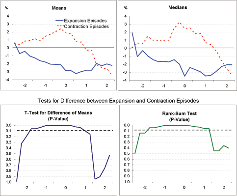
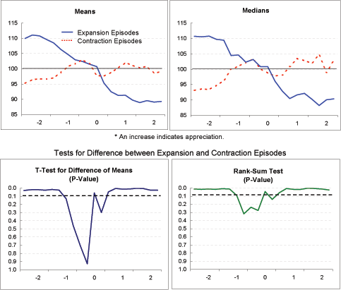
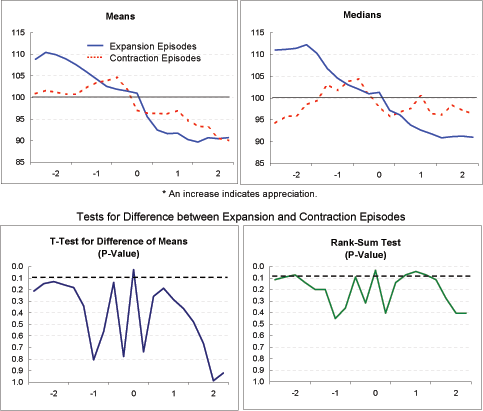
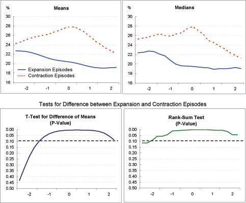
Real effective exchange rate (Exhibit 4f): The two groups exhibit surprisingly (and very significantly) different trends for this indicator. Among the expansion episodes, the real exchange rate depreciates through most of the period, consistent with the view that depreciation leads to current account adjustment with a lag of several years. Among the contraction episodes, the real exchange rate is essentially unchanged over the period, suggesting that something else besides changes in relative prices-most likely a compression of domestic demand-is responsible for current account adjustment.

Nominal effective exchange rate (Exhibit 4g): For the expansion episodes, the real depreciation indicated in Exhibit 4f clearly reflects nominal depreciation (rather than a fall in national price levels). For the contraction episodes, especially based on the means, some nominal depreciation is apparent between the beginning of Year 0 and Year 2. The fact that this nominal depreciation did not translate into sustained real depreciation is explained by the higher inflation among the contraction episodes, shown in Exhibit 4e. Additionally, for the period as a whole (Year -2 to Year 2), the expansion episodes clearly evidence more nominal depreciation than the contraction episodes; in fact, for the median measure, the nominal exchange rate for the contraction episodes rises slightly on balance.

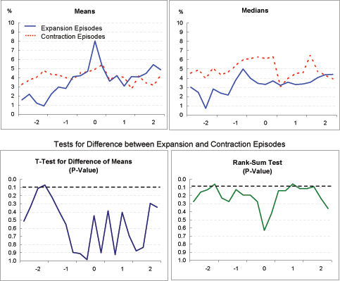
Real policy interest rate (Exhibit 4h): There appears to be some tendency for rates to move up before current account adjustment in both groups and move down thereafter, although the mean and median measures do not track each other closely for this indicator. In neither group is there much evidence of a sharp increase in real policy rates with the initiation of current account adjustment. Moreover, interest rates move relatively similarly in the two groups.

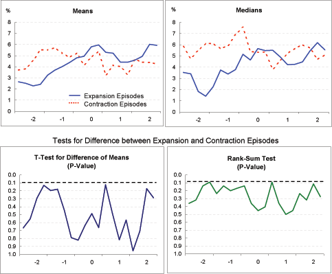
Real long-term interest rate (Exhibit 4i): As with real policy rates, there is some tendency for real long-term rates to rise prior to current account adjustment and to fall thereafter. The decline seems more marked for the contraction episodes than the expansion episodes, possibly owing to the weaker growth in the former group, but for the most part differences between the two groups are not statistically significant.

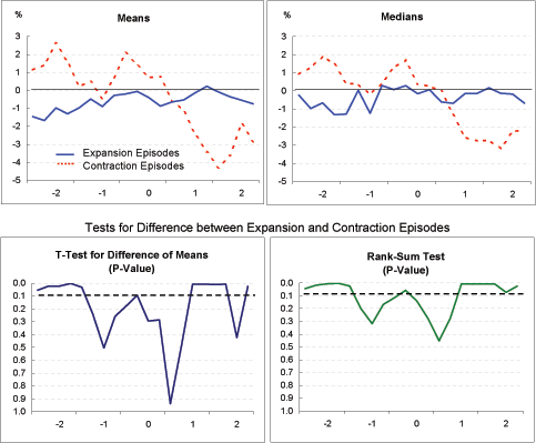
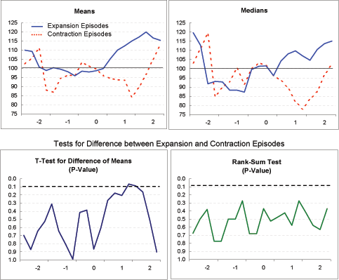
Real stock market price (Exhibit 4j): Both for the expansion and contraction group, real stock market prices appear to decline, on balance, between the beginning of Year -2 and Year 0. With the onset of current account adjustment, real stock prices in the expansion episodes trend upward, whereas prices in the contraction episodes fall sharply before rebounding. This sharp decline in stock prices among the contraction episodes in Years 0 and 1 is, indeed, consistent with the disorderly adjustment hypothesis, except that it is not associated with real exchange rate depreciation. Conversely, among the expansion episodes, there is considerable exchange rate depreciation, but this appears to come after stock prices have declined. In any event, notwithstanding the important differences in the evolution of GDP growth between the expansion and contraction episodes, stock price indexes in the two groups generally are not significantly different from each other.

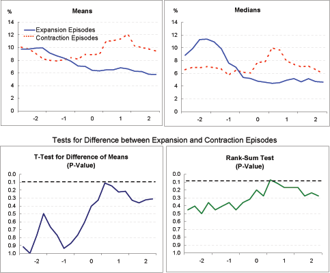
Saving and investment ( Exhibits 4k, 4l): Saving and investment rates move quite differently across the adjustment period in the expansion and contraction episodes. In the contraction episodes, adjustment is preceded by increases in investment rates that outstrip increases in saving; subsequently, current account adjustment is driven by a sharp decline in investment rates which more than offsets a smaller fall in saving rates. In the expansion episodes, both investment and saving rates appear to decline prior to the onset of current account adjustment, with saving rates falling a bit more than investment rates; subsequent current account adjustment appears to be achieved through a combination of higher saving rates and somewhat lower investment rates. Thus, while for the entire sample of adjustment episodes, as documented in Section II above, current account adjustment appears mainly to reflect reductions in investment spending, this finding does not apply to those episodes exhibiting the greatest increases in GDP growth.

Real imports and exports (Exhibits 4m, 4n, 4o): Notwithstanding the fact that the expansion episodes were associated with considerable real exchange rate depreciation whereas the contraction episodes were not, both groups exhibited steady growth of real exports (Exhibit 4m) before and after the onset of current account adjustment, although growth is a bit faster for the expansion episodes. It is in the behavior of imports (Exhibit 4n) that the two groups differ importantly. The expansion episodes exhibit some continued import growth after the onset of current account adjustment, in spite of the real depreciation of the exchange rate, no doubt driven by the pickup in GDP growth. Conversely, in the contraction episodes, imports stall and even edge down somewhat, consistent with the decline in GDP among these economies.

Considering that export growth among the expansion and contraction episodes is similar, while import growth is higher among the expansion episodes than the contraction episodes, it may seem curious that both groups of episodes exhibit a similar extent of current account adjustment, measured as a share of GDP (Exhibit 4a). This seeming contradiction is reconciled by the fact that the ratio of imports to exports is much lower among the expansion episodes than the contraction episodes (Exhibit 4o). For a given growth rate of exports and imports, the smaller the ratio of imports to exports, the larger the reduction in the trade deficit. Thus, the expansion episodes are able to achieve the same degree of current account adjustment as the contraction episodes, but with less import compression.

Budget balance (Exhibits 4p, 4q): The expansion and contraction episodes exhibit very different patterns in the evolution of their budget balances (Exhibit 4p). The expansion episodes exhibit an increase in deficits up until the onset of current account adjustment, followed by a movement toward balance; this is consistent with the "twin deficits" hypothesis. Conversely, the contraction episodes evidence the reverse, with budget surpluses rising and the falling. These patterns appear to be statistically significantly different from each other.

However, differences in the evolution of budget balances appear to be driven by movements in GDP growth. The cyclically-adjusted budget balances (Exhibit 4q) evidence murkier patterns for both types of episodes, but ones that are not significantly different from each other.

Net international investment position (Exhibit 4r): The NIIP for the expansion episodes appears fairly stable over the period while that for the contraction episodes moves down, consistent with the larger current account deficits in the latter group. However, on account of the wide dispersion of NIIPs, differences between the groups are not statistically significant.

4  Correlations Among Indicators Across All Episodes

An alternative approach to gauging the factors influencing GDP growth during current account adjustments is to examine the correlation between growth and other economic indicators across all 23 episodes in our sample. Exhibit 5 presents the results of this analysis, which focuses on the linkages in the data between GDP growth and several key indicators. By and large, the results confirm the findings described in the previous section and further contradict the predictions of the disorderly correction hypothesis.

Exhibit 5a plots the percent increase (appreciation) in the real exchange rate from before to after the current account reached its trough-the X axis-against the percentage point increase in GDP growth over the same period-the Y axis. It makes clear that among the adjustment episodes in our sample, the greater the extent of real exchange rate depreciation, the larger the increase in GDP growth over the period.

Exhibit 5b plots the increase in the current account/GDP ratio from before to after this ratio bottomed out-the X axis-against the increase in GDP growth-the Y axis. Contrary to the predictions of "adjustment pessimists", greater reductions in the current account deficit are associated with higher, not lower, GDP growth. This correlation remains positive and about the same magnitude when the outlier in the bottom left quadrant of the scatterplot was excluded (not shown).

Exhibit 5c shows that increases in the real long-term interest rate from before to after the current account balance troughs are, again, associated with higher, not lower, GDP growth. Contrary to the predictions of the disorderly correction hypothesis-that adjustment will prompt a surge in interest rates that depresses GDP-causation most likely was operating in the opposite direction: higher GDP growth led to higher real interest rates.

Exhibit 5d provides some evidence that changes in GDP growth are correlated with changes in real stock prices, although the slope coefficient for the regression line (not shown) is not significantly different from zero. However, it is not obvious that causality runs exclusively from stock prices to GDP. Moreover, and, again, contrary to the disorderly correction hypothesis, almost half the observations involve increases in real stock prices during the adjustment period.

The final two panels in Exhibit 5 address the importance of two key initial conditions. Exhibit 5e indicates that the greater the current account deficit at its trough in Year 0, the lesser the rise in growth rates from before to after the onset of adjustment. This finding is consistent with that shown in Exhibit 4a, which indicates a narrower current account deficit for the expansion episodes than the contraction episodes. However, the most obvious interpretation of this finding-that the larger the deficit, the greater the needed adjustment and hence the lesser the GDP growth-may not be correct. Both the expansion and contraction episodes evidenced similar amounts of adjustment, and moreover, Exhibit 5b shows that improvements in the current account are positively correlated with changes in GDP growth. An alternative interpretation is that historically, those economies experiencing the greatest degree of overheating evidenced the largest current account deficits and the greatest subsequent contraction in GDP growth.

Finally, Exhibit 5f shows that there is little correlation between an economy's net international investment position and the change in growth of GDP. (The slope coefficient, not shown, of the regression line is only -0.03 with a t-statistic of -0.73).

5  Robustness Analysis

The approach we have taken to sorting the episodes into the expansion and contraction groups is, to a certain extent, arbitrary. As mentioned in Section III, we used the change in the four-quarter growth of real GDP from the averages of Years -2 and -1 to the averages of Years 1 and 2 to sort the episodes into the two groups. To assess the sensitivity of our results to this sorting mechanism, we conduct two alternative calculations. In the first one, we continue to use the change in the four-quarter growth of real GDP, but compute the change in growth rates from the average for the three years preceding the current account reversal to the three years after the reversal.¹³ Our second alternative sorting mechanism uses the change in 2-year averages of year-over-year GDP growth rates rather than four-quarter growth rates.¹⁴ Exhibits 6a and 6b show the results for four main indicators of interest under these two alternative calculations.

Exhibit 6a confirms that lengthening the time span used to calculate average GDP growth rates from two years to three years (in order to distinguish expansion and contraction episodes) has little effect on the behavior of these indicators. The contraction episodes are still characterized by little change in the real exchange rate and a significant fall in GDP growth that starts before the current account adjustment and lowers imports demand. Moreover, a notable depreciation of the real exchange rate initiated prior to the adjustment continues to typify the expansion episodes. The t-test and rank-sum test corroborate that the difference between the expansion and contraction episodes remains significant.

We find that sorting the episodes using changes in year-over-year GDP growth does not significantly affect our main findings, either. Exhibit 6b shows that although GDP growth is now a bit more similar for the expansion and contraction episodes two years before the reversal, the overall picture for GDP growth remains the same. As before, the real exchange rate is about constant throughout the adjustment process for the contraction episodes, while it depreciates for the expansion episodes. However, the difference between the two paths is not as significant as under our original calculation.

Finally, changing the sorting mechanism did not affect the behavior of the stock market and interest rates (not shown) over the adjustment process. We continue to find no evidence that current account reversals are associated with sharp declines in asset prices.

6  Conclusion

In this paper, we reviewed the experience of 23 current account adjustment episodes in industrialized economies, building on previous work in this area by Freund (2000). In order to assess the possible disruptive effects of adjustment, and to gain a sense of the factors associated with such disruption, we identified two sub-samples of these episodes: those exhibiting the largest increases in real GDP growth from before to after the onset of adjustment, and those exhibiting the largest declines in growth. We then compared the paths of key performance indicators in the two groups and assessed the extent to which the behavior of these indicators, particularly in the contraction episodes, resembled that described in the disorderly correction scenario.

Our main findings are as follows. First, a significant subset of the adjustment episodes we studied were associated with substantial declines in GDP growth. For the seven contraction episodes (those experiencing the largest decline in growth between the two years preceding the onset of current account adjustment and the two years following), median 4-quarter GDP growth registered under 1 percent in the first year after adjustment started and -1/2 percent in the second. Thus, the fear that current account adjustment might be associated with recession is not entirely without basis.

However, our second main finding is that the shortfall in growth experienced in the contraction episodes appears to reflect the playing out of standard cyclical developments rather than a response to current account adjustment. Prior to current account adjustment, these episodes were characterized by growth in excess of potential, a consequent rise in the level of output relative to potential, and a widening of the current account balance. In the years after the current account reached its trough and started to correct, GDP growth declined and output fell below potential.

These shortfalls in growth are not consistent with the disorderly adjustment scenario (a fall in the currency that pushes up interest rates, depresses stock prices, reduces net worth, and induces a recession). The contraction episodes evidenced no decline in real exchange rates, and only mixed indications of a decline in nominal exchange rates, over the period; apparently, adjustment was accomplished exclusively through reductions in domestic demand that compressed imports. Moreover, neither long-term real interest rates nor real stock market prices moved in a significant and sustained adverse direction during the period.

Our third main finding is that among those episodes that experienced the largest increases in growth from before to after the onset of current account adjustment-the expansion episodes-the reduction in external deficits owed significantly to changes in exchange rates rather than merely compression of domestic demand. Real exchange rate depreciation commenced in the year prior to the onset of current account adjustment and extended through at least the year after the onset. With GDP growth on the rise as well, current account adjustment was achieved through export growth that exceeded still-positive import growth, rather than through the compression of imports evidenced by the contraction episodes.

Importantly, during the time-frame we examined, the expansion episodes evidenced very low levels of growth (and apparently substantially below potential) as well, but in the years prior to current account adjustment rather than in the years after the onset of adjustment. As these shortfalls in growth also preceded the fall in real currency values, they are inconsistent with the disorderly correction scenario. In fact, our surmise is that shortfalls in growth led to declines in currency values rather than vice-versa.

The results of our analysis were generally robust to alternative means of sorting the episodes into expansion and contraction episodes. These results were also confirmed by analysis of correlations among performance indicators across all 23 adjustment episodes in our sample. Contrary to the predictions of the disorderly correction hypothesis, changes in GDP growth rates from before to after the onset of current account adjustment were positively correlated with the extent of exchange rate depreciation as well as with increases in long-term real interest rates. Changes in GDP growth were negatively correlated with the initial size of the current account deficit, but positively related to the extent of subsequent current account adjustment. Finally, GDP growth appears not to have been correlated with the initial net international investment position of the economy.

It should be emphasized that these findings do not "disprove" the disorderly adjustment hypothesis. We have not estimated the structural relationships linking exchange rates, other asset prices, and economic activity, nor have we used the results of such estimates to reject the hypothesis that current account adjustment may induce financial and economic disruptions. Thus, we cannot rule out the possibility that, under certain circumstances, the correction of external imbalances may, indeed, be disruptive.

However, we have shown that, among historical episodes of adjustment in industrialized countries, there has been little evidence of the pattern of developments described by the disorderly correction scenario. Thus, our findings suggest that there is little historical basis for the view that current account adjustment poses a threat to U.S. economic growth.

Although our findings provide some grounds for optimism about the implications of current account adjustment, several cautions should be noted. First, it is unclear how predictive the experience of foreign economies undergoing current account adjustment is for U.S. economic prospects. The U.S. economy is the largest economy in the world, with the greatest potential to affect the growth of its trading partners; it is generally less open than the other economies in the sample; we issue the world's most prominent reserve currency; and our product, labor, and financial markets are generally considered to be exceptionally flexible. The implications of these differences, on balance, are not clear-cut. Note, however, that the U.S. current account adjustment of the late 1980s is the only episode in the sample in which GDP growth exceeded 2 $\raise.5ex\hbox{$\scriptstyle 1$}\kern-.1em/ \kern-.15em\lower.25ex\hbox{$\scriptstyle 2$}$ percent before, during, and after the onset of current account adjustment.

Second, as noted above, even in the expansion episodes, very low levels of growth were registered, albeit prior to rather than during current account adjustment. These shortfalls in growth do not appear attributable to exchange rate depreciation. Nevertheless, it remains unclear why these shortfalls took place and whether they might, in some way, have been necessary for subsequent external imbalance correction.

Finally, the U.S. current account deficit, at present, is already larger than it was for the average of the episodes in our sample. To some extent, of course, the large and growing deficit is a reflection of the financial markets' decisions as to where to allocate global savings. However, the size of the deficit likely increases the extent of external adjustment that might be required in the future. On the one hand, this could mean greater dislocations in financial markets and economic activity during the adjustment process. On the other hand, as noted above, we found no evidence that episodes with greater degrees of current account adjustment also experienced larger shortfalls in GDP growth.

Data Appendix

All data is from the OECD National Accounts and Main Economic Indicators in local currency on a quarterly basis except for saving, investment and the structural government budget balance (as a percent of potential GDP) which are on an annual basis. Data on the structural budget balance were not available from this source for the Denmark, New Zealand, and Sweden (1982) episodes.

The harmonized CPI is used for the EU countries.

The real effective exchange rate from the BIS is the nominal effective exchange rate adjusted for changes in consumer prices.

The real policy and long interest rates are nominal rates adjusted with the 4-quarter change in the headline CPI and similarly for the real stock market index. Stock market data were not available for the Greece (1985) episode.

The annual net international investment position data are from the IMF Balance of Payments Statistics. Data were not available from this source for the Austria (1980), Denmark, Greece, Ireland, New Zealand, Portugal, Spain (1981) and Sweden (1982) episodes.

References

Ahmed, S., C. Gust, J. Huntley and S. Kamin, 2002. "Are Depreciations as Contractionary as Devaluations? A Comparison of Selected Emerging and Industrial Economies," Board of Governors of the Federal Reserve System International Finance Discussion Papers 2002-737.

Bank for International Settlements, 2004. 74$^{th}$ Annual Report.

Calvo, Guillermo and Carmen M. Reinhart. 2001. "Fixing for Your Life," in Susan M. Collins and Dani Rodrik, eds., Brookings Trade Forum: 2000, Brookings Institution Press, Washington, D.C.

Diaz-Alejandro, Carlos. 1963. "A Note on the Impact of Devaluation and Redistributive Effects,"Journal of Political Economy 71, 577-580.

Edwards, S., 2004. "Thirty Years of Current Account Imbalances, Current Account Reversals, and Sudden Stops," IMF Staff Papers 51, 1-49.

The Economist. 2004. "Special Report: The Future of the Dollar," December 4.

Eichengreen, Barry. 2004. "Why the Dollar's Fall is Not to be Welcomed," Financial Times, December 20.

Fligner, M.A. and Pollicello, G.E. III, 1981. "Robust Rank Procedures for Behrens-Fisher Problem," Journal of the American Statistical Association 76, 162-168.

Freund, C., 2000. "Current Account Adjustment in Industrial Countries," Board of Governors of the Federal Reserve System International Finance Discussion Papers 2000-693.

Hatzius, Jan., 2004. "All Eyes on the Trade Balance in 2005," Goldman Sachs Group Inc. US Economics Analyst: New York, December 31.

International Monetary Fund, September 2002. World Economic Outlook.

Krugman, Paul and Lance Taylor. 1978. "Contractionary Effects of Devaluation," Journal of International Economics 8, 445-456.

Lizondo, Saul and Peter Montiel. 1989. "Contractionary Effects of Devaluation in Developing Countries: An Analytical Overview," IMF Staff Papers 36, 182-227.

Mann, C.L., 1999. "Is the U.S. Trade Deficit Sustainable?" Institute For International Economics, Washington, D.C.

Mann, C.L., 2002. "Perspectives on the U.S. Current Account Deficit and Sustainability," Journal of Economic Perspectives 16, 131-152.

Milesi-Ferretti, G.M. and A. Razin, 2000. "Current Account Reversals and Currency Crises: Empirical Regularities," in P. Krugman, ed., Currency Crises, The University of Chicago Press: Chicago and London, 285-325.

Mussa, Michael. 2004. "Exchange Rate Adjustments Needed to Reduce Global Payments Imbalances," in C. Fred Bergstrom and John Williamson, eds.,Dollar Adjustment: How Far? Against Whom?, Institute for International Economics: Washington, D.C., 113-138.

Obstfeld, M. and K. Rogoff, 2004. "The Unsustainable US Current Account Position Revisited," National Bureau of Economic Research Working Paper 10869.

Ragan, Raghuram. 2004. Remarks at the Australasian Finance and Banking Conference. Sydney, Australia, December 15.

Roubini, N. and B. Setser, 2004. "The US as a Net Debtor: The Sustainability of the US External Imbalances," manuscript.

Tilton, Andrew. 2005. "Who Will Benefit From Trade Improvement?" Goldman Sachs Group Inc. US Economics Analyst: New York, January 21.

Truman, Edwin. 2004. "Budget and External Deficits: Same Family but not Twins," prepared for Federal Reserve Bank of Boston Annual Research Conference, The Macroeconomics of Fiscal Policy, June 14-16.

Wolf, Martin, 2004. "The World Has a Dangerous Hunger for American Assets," Financial Times, December 8.

Exhibit 1

Country	Year 0	CA-GDP Ratio Year 0	CA-GDP Ratio Year +2
Australia	1989	-6.11	-3.53
Austria	1980	-2.08	1.03
Austria	1999	-3.05	-1.93
Belgium	1980	-3.09	-1.15
Canada	1981	-4.16	-0.74
Canada	1993	-3.86	-0.76
Denmark	1986	-5.45	-1.45
Finland	1991	-5.48	-1.38
France	1982	-1.99	-0.19
Greece	1985	-9.33	-3.12
Greece	1990	-5.69	-3.58
Ireland	1981	-13.07	-5.90
Italy	1981	-2.44	0.20
Italy	1992	-2.31	1.23
New Zealand	1984	-8.40	-6.56
Norway	1986	-6.27	-4.09
Portugal	1982	-11.46	-2.64
Spain	1981	-3.04	-2.04
Spain	1991	-3.64	-1.09
Sweden	1982	-2.98	0.51
Sweden	1992	-2.81	1.08
UK	1989	-5.12	-1.82
US	1987	-3.39	-1.82
Median	All	-3.86	-1.45
Mean	All	-5.01	-1.73

Exhibit 2:  Indicator Averages Across All Episodes

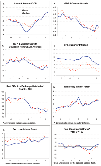
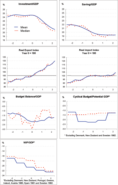
Exhibit 3:  Real GDP 4-Quarter Growth

Episode	Year	Change*	Year -2	Year -1	Year 0	Year +1	Year +2
Sweden	1992	5.15	0.92	-1.59	-4.07	4.45	5.16
Sweden	1982	3.67	-0.38	0.53	0.94	3.35	4.14
Canada	1993	3.20	-0.53	0.90	2.96	5.41	1.39
Spain	1981	1.03	0.59	0.96	-0.34	1.83	1.79
Italy	1992	0.47	-0.36	2.76	-1.10	0.55	2.79
US	1987	-0.35	4.17	2.84	4.48	3.66	2.66
France	1982	-0.36	0.45	2.53	1.73	1.15	1.10
Finland	1991	-0.56	3.61	-3.51	-6.82	-2.33	1.22
Austria	1980	-1.51	-1.17	6.03	0.62	-0.38	2.11
Canada	1981	-1.57	3.63	1.79	2.20	-3.71	6.24
Austria	1999	-1.57	2.95	2.86	3.64	2.89	-0.20
Ireland	1981	-1.79	2.23	2.43	2.61	0.46	0.63
Greece	1985	-2.30	-0.23	2.78	2.29	-1.31	-0.75
Italy	1981	-2.38	6.54	1.54	0.46	-0.70	4.02
Belgium	1980	-2.48	3.01	3.14	-1.95	1.32	-0.12
Greece	1990	-2.67	6.06	1.64	0.63	3.43	-1.08
Denmark	1986	-3.39	3.20	5.50	1.44	0.26	1.65
Portugal	1982	-3.58	2.98	0.90	4.61	-2.99	-0.27
New Zealand	1984	-4.35	4.22	3.88	7.32	1.09	-1.66
Australia	1989	-4.48	5.90	3.41	3.64	0.82	-0.48
Norway	1986	-4.78	5.72	4.47	3.27	1.71	-1.07
UK	1989	-5.07	4.81	4.23	1.11	-0.44	-0.66
Spain	1991	-5.50	4.58	6.15	0.52	-0.91	0.63

*  Episodes were ranked according to the change in growth from Year -2 and Year -1 to Year +1 and Year +2.

Exhibit 4a:  Current Account / GDP

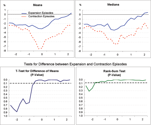
Exhibit 4b:  Real GDP 4-Quarter Growth

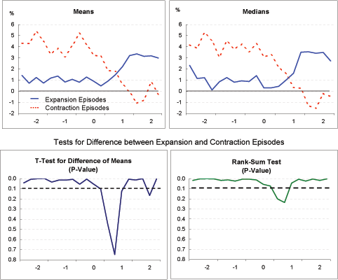
Exhibit 4c:  Output Gap

Data for Exhibit 4c

Year	Quarter	Means: Expansion	Means: Contraction	Medians: Expansion	Medians: Contraction	T-Test for Difference of Means	Rank-Sum Test
-2	1	0.6	0.6	1.9	0.0	0.99	0.50
-2	2	-0.7	0.4	-1.1	0.7	0.32	0.14
-2	3	-0.4	0.9	-0.3	0.6	0.19	0.14
-2	4	-1.0	1.0	-1.0	1.5	0.06	0.04
-1	1	-1.3	1.2	-1.4	1.0	0.06	0.04
-1	2	-1.6	0.9	-1.7	1.0	0.03	0.02
-1	3	-1.8	1.4	-1.6	1.0	0.01	0.00
-1	4	-2.0	1.7	-1.7	1.0	0.00	0.00
0	1	-2.1	2.0	-1.4	2.5	0.01	0.01
0	2	-2.1	2.4	-2.0	3.2	0.00	0.01
0	3	-2.9	1.9	-3.5	2.5	0.00	0.00
0	4	-2.9	1.8	-2.4	2.5	0.00	0.01
1	1	-3.2	0.8	-2.7	1.8	0.03	0.02
1	2	-3.0	0.7	-2.9	1.8	0.04	0.03
1	3	-2.8	-0.3	-3.5	0.7	0.10	0.06
1	4	-2.8	-0.3	-3.4	0.4	0.16	0.06
2	1	-2.0	-2.1	-2.9	-0.3	0.95	0.45
2	2	-2.2	-2.5	-2.3	-1.5	0.91	0.45
2	3	-2.0	-2.6	-2.1	-2.6	0.75	0.36
2	4	-2.2	-3.4	-2.1	-3.4	0.53	0.40

Exhibit 4d:  Deviation from OECD Average Real GDP 4-Quarter Growth

Data for Exhibit 4d

Year	Quarter	Means: Expansion	Means: Contraction	Medians: Expansion	Medians: Contraction	T-Test for Difference of Means	Rank-Sum Test
-2	1	-1.5	1.1	-0.2	0.9	0.05	0.04
-2	2	-1.7	1.4	-1.0	1.3	0.02	0.02
-2	3	-1.0	2.6	-0.7	1.9	0.02	0.01
-2	4	-1.3	1.6	-1.3	1.5	0.00	0.00
-1	1	-1.0	0.2	-1.3	0.4	0.03	0.02
-1	2	-0.5	0.5	0.0	0.4	0.24	0.20
-1	3	-0.9	-0.4	-1.2	-0.2	0.50	0.32
-1	4	-0.3	0.7	0.3	0.4	0.26	0.17
0	1	-0.2	2.1	0.1	1.3	0.18	0.11
0	2	-0.1	1.4	0.3	1.7	0.09	0.06
0	3	-0.4	0.7	-0.2	0.4	0.30	0.14
0	4	-0.9	0.8	0.1	0.3	0.29	0.28
1	1	-0.6	-0.6	-0.6	0.0	0.94	0.45
1	2	-0.5	-1.1	-0.7	-1.3	0.48	0.28
1	3	-0.1	-2.5	-0.1	-2.6	0.01	0.01
1	4	0.2	-3.4	-0.1	-2.8	0.01	0.01
2	1	-0.1	-4.3	0.2	-2.7	0.01	0.01
2	2	-0.4	-3.6	-0.1	-3.2	0.01	0.01
2	3	-0.5	-1.8	-0.2	-2.2	0.42	0.07
2	4	-0.7	-2.8	-0.7	-2.1	0.02	0.02

Exhibit 4e:  CPI 4-Quarter Inflation

Data for Exhibit 4e

Year	Quarter	Means: Expansion	Means: Contraction	Medians: Expansion	Medians: Contraction	T-Test for Difference of Means	Rank-Sum Test
-2	1	9.7	10.1	8.8	6.6	0.92	0.45
-2	2	9.7	9.7	9.9	7.0	1.00	0.40
-2	3	9.9	9.1	11.3	6.9	0.77	0.50
-2	4	10.0	8.2	11.4	7.1	0.50	0.36
-1	1	9.1	8.0	10.9	6.9	0.67	0.45
-1	2	8.7	7.9	9.8	6.7	0.77	0.40
-1	3	8.3	8.1	7.6	5.7	0.94	0.36
-1	4	7.8	8.4	7.0	6.5	0.87	0.45
0	1	7.1	8.2	5.4	6.2	0.77	0.36
0	2	7.0	8.9	5.2	6.1	0.61	0.32
0	3	6.4	8.9	4.8	7.7	0.40	0.20
0	4	6.3	9.0	4.6	7.8	0.33	0.28
1	1	6.5	11.0	4.4	10.0	0.11	0.07
1	2	6.5	11.1	4.5	9.6	0.15	0.11
1	3	6.8	11.4	4.9	7.9	0.22	0.17
1	4	6.6	12.1	5.2	7.4	0.21	0.17
2	1	6.3	10.3	4.7	7.0	0.33	0.17
2	2	6.2	10.0	5.2	7.2	0.36	0.28
2	3	5.8	9.8	4.7	6.6	0.32	0.24
2	4	5.8	9.4	4.6	6.0	0.31	0.28

Exhibit 4f:  Real Effective Exchange Rate
Index Year 0 = 100

Data for Exhibit 4f

Year	Quarter	Means: Expansion	Means: Contraction	Medians: Expansion	Medians: Contraction	T-Test for Difference of Means	Rank-Sum Test
-2	1	110.0	95.2	110.7	93.1	0.03	0.01
-2	2	111.1	96.4	110.6	93.6	0.02	0.02
-2	3	110.8	96.7	110.8	93.4	0.02	0.01
-2	4	109.6	96.7	109.7	94.7	0.03	0.02
-1	1	108.5	97.0	109.4	96.3	0.02	0.01
-1	2	106.3	98.8	104.5	99.9	0.03	0.01
-1	3	104.7	100.8	104.6	101.0	0.13	0.09
-1	4	103.0	101.7	102.3	102.1	0.46	0.32
0	1	102.4	103.0	103.2	103.3	0.70	0.24
0	2	101.5	101.6	100.8	100.1	0.93	0.28
0	3	100.7	97.8	100.8	98.8	0.06	0.04
0	4	95.3	97.6	96.1	97.8	0.30	0.14
1	1	92.5	98.9	92.8	98.2	0.05	0.06
1	2	91.3	100.3	90.5	100.9	0.00	0.01
1	3	91.3	102.0	91.6	103.4	0.01	0.02
1	4	89.7	101.1	92.2	102.8	0.01	0.02
2	1	88.9	100.3	90.3	102.0	0.00	0.00
2	2	89.5	100.8	88.2	104.7	0.01	0.01
2	3	89.1	98.6	90.0	99.0	0.03	0.01
2	4	89.3	99.1	90.4	102.8	0.03	0.02

Exhibit 4g:  Nominal Effective Exchange Rate
Index Year 0 = 100

Data for Exhibit 4g

Year	Quarter	Means: Expansion	Means: Contraction	Medians: Expansion	Medians: Contraction	T-Test for Difference of Means	Rank-Sum Test
-2	1	108.9	100.9	111.1	94.3	0.21	0.11
-2	2	110.4	101.6	111.2	95.8	0.15	0.09
-2	3	109.9	101.2	111.4	95.9	0.13	0.07
-2	4	108.9	100.8	112.3	98.5	0.16	0.14
-1	1	107.6	100.7	110.3	99.4	0.18	0.20
-1	2	106.0	102.2	106.8	103.1	0.34	0.20
-1	3	104.3	103.5	104.5	101.8	0.81	0.45
-1	4	102.6	103.9	103.0	103.8	0.56	0.36
0	1	101.9	104.6	102.1	104.3	0.14	0.09
0	2	101.5	102.0	101.0	100.7	0.78	0.32
0	3	101.0	97.1	101.3	98.1	0.03	0.03
0	4	95.6	96.4	97.2	95.8	0.74	0.40
1	1	92.5	96.3	96.1	96.8	0.26	0.14
1	2	91.6	96.2	93.8	97.7	0.19	0.07
1	3	91.7	97.0	92.6	100.5	0.29	0.04
1	4	90.3	94.7	91.8	96.5	0.36	0.07
2	1	89.7	93.4	90.9	96.2	0.48	0.11
2	2	90.7	93.1	91.1	98.4	0.66	0.28
2	3	90.5	90.6	91.3	97.1	0.99	0.40
2	4	90.7	90.1	91.0	96.4	0.92	0.40

Exhibit 4h:  Real Policy Interest Rate

Data for Exhibit 4h

Year	Quarter	Means: Expansion	Means: Contraction	Medians: Expansion	Medians: Contraction	T-Test for Difference of Means	Rank-Sum Test
-2	1	1.6	3.2	3.0	4.5	0.51	0.27
-2	2	2.2	3.8	2.5	4.9	0.33	0.16
-2	3	1.2	4.0	0.7	4.0	0.11	0.13
-2	4	0.9	4.8	2.8	5.1	0.07	0.06
-1	1	2.2	4.4	2.4	4.4	0.22	0.23
-1	2	3.0	4.3	2.2	4.6	0.39	0.27
-1	3	2.8	4.0	3.8	5.4	0.55	0.13
-1	4	4.1	3.8	5.0	6.0	0.90	0.19
0	1	4.2	4.5	4.0	6.1	0.91	0.19
0	2	4.7	4.6	3.4	6.3	0.98	0.27
0	3	8.0	4.9	3.3	6.1	0.45	0.63
0	4	5.2	5.5	3.7	6.3	0.90	0.42
1	1	3.6	3.8	3.2	3.1	0.39	0.14
1	2	4.2	4.2	3.6	3.9	0.92	0.14
1	3	3.1	4.0	3.3	4.5	0.40	0.06
1	4	4.1	2.8	3.4	4.6	0.69	0.11
2	1	4.1	4.2	3.6	6.4	0.88	0.11
2	2	4.5	3.4	4.1	4.8	0.83	0.09
2	3	5.4	3.2	4.4	4.3	0.29	0.24
2	4	4.9	4.2	4.4	3.9	0.34	0.36

Exhibit 4i:  Real Long Interest Rate

Data for Exhibit 4i

Year	Quarter	Means: Expansion	Means: Contraction	Medians: Expansion	Medians: Contraction	T-Test for Difference of Means	Rank-Sum Test
-2	1	2.6	3.7	3.5	5.8	0.67	0.36
-2	2	2.5	3.8	3.4	4.8	0.55	0.32
-2	3	2.3	4.5	1.8	5.5	0.29	0.14
-2	4	2.4	5.5	1.4	6.1	0.13	0.09
-1	1	3.3	5.5	2.3	6.1	0.20	0.24
-1	2	3.7	5.7	3.8	5.7	0.18	0.14
-1	3	4.0	5.2	3.4	5.9	0.45	0.20
-1	4	4.4	4.9	3.8	6.9	0.79	0.17
0	1	4.8	5.2	5.2	7.6	0.82	0.14
0	2	5.0	4.2	4.6	5.4	0.64	0.36
0	3	5.8	4.9	5.7	5.3	0.49	0.45
0	4	6.0	5.4	5.5	5.4	0.66	0.40
1	1	5.3	3.3	5.5	3.8	0.12	0.09
1	2	5.2	4.1	4.9	4.6	0.49	0.36
1	3	4.4	4.0	4.2	5.2	0.82	0.50
1	4	4.4	3.3	4.3	5.7	0.57	0.45
2	1	4.6	4.7	4.5	6.0	0.96	0.24
2	2	4.9	4.4	5.4	5.7	0.71	0.32
2	3	6.0	4.4	6.2	4.7	0.17	0.11
2	4	5.9	4.3	5.6	5.1	0.29	0.28

Exhibit 4j:  Real Stock Market Index
Year 0 = 100

Data for Exhibit 4j

Year	Quarter	Means: Expansion	Means: Contraction	Medians: Expansion	Medians: Contraction	T-Test for Difference of Means	Rank-Sum Test
-2	1	110.0	102.4	119.6	103.2	0.70	0.67
-2	2	109.2	105.7	112.7	111.0	0.87	0.50
-2	3	100.7	111.2	91.8	119.4	0.64	0.38
-2	4	98.8	88.1	93.1	84.8	0.53	0.77
-1	1	100.3	86.8	92.8	89.8	0.31	0.77
-1	2	99.5	94.3	88.3	93.1	0.64	0.50
-1	3	98.2	96.2	88.3	100.4	0.81	0.50
-1	4	95.9	96.0	87.2	91.5	0.99	0.27
0	1	98.4	103.1	99.6	99.9	0.41	0.68
0	2	97.9	101.3	101.4	103.2	0.39	0.68
0	3	98.7	99.5	101.5	101.7	0.87	0.37
0	4	99.9	96.0	96.2	96.3	0.61	0.53
1	1	105.3	94.4	104.1	93.6	0.27	0.47
1	2	110.0	93.7	108.1	89.5	0.18	0.42
1	3	112.3	93.4	109.7	82.1	0.21	0.58
1	4	115.0	84.2	107.0	78.0	0.07	0.27
2	1	117.1	89.4	104.7	83.3	0.09	0.42
2	2	119.9	96.7	110.5	87.4	0.16	0.58
2	3	116.7	105.0	113.7	96.6	0.51	0.63
2	4	115.4	112.8	115.1	102.5	0.90	0.37

Exhibit 4k:  Investment / GDP

Data for Exhibit 4k

Year	Quarter	Means: Expansion	Means: Contraction	Medians: Expansion	Medians: Contraction	T-Test for Difference of Means	Rank-Sum Test
-2	1	22.7	24.2	22.4	25.3	0.43	0.11
-2	2	22.7	24.7	22.5	25.5	0.33	0.11
-2	3	22.6	25.1	22.7	25.7	0.23	0.09
-2	4	22.3	25.5	22.6	26.1	0.15	0.06
-1	1	22.0	25.8	22.1	26.4	0.10	0.06
-1	2	21.6	26.0	21.7	26.0	0.06	0.04
-1	3	21.2	26.2	20.8	25.9	0.04	0.01
-1	4	20.9	26.6	20.0	26.3	0.02	0.01
0	1	20.7	27.0	19.6	26.6	0.01	0.01
0	2	20.5	27.5	19.6	27.4	0.01	0.00
0	3	20.4	27.8	19.5	27.9	0.00	0.00
0	4	20.2	27.8	19.4	27.3	0.00	0.00
1	1	19.9	27.4	19.3	26.3	0.00	0.00
1	2	19.6	26.7	19.2	25.0	0.00	0.00
1	3	19.4	25.8	18.9	24.5	0.01	0.00
1	4	19.2	24.9	19.0	23.9	0.01	0.01
2	1	19.1	24.1	19.0	23.2	0.01	0.01
2	2	19.1	23.3	19.1	22.5	0.03	0.02
2	3	19.1	22.7	19.3	21.8	0.05	0.04
2	4	19.2	22.2	19.0	21.3	0.09	0.04

Exhibit 4l:  Saving / GDP

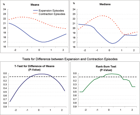
Data for Exhibit 4l

Year	Quarter	Means: Expansion	Means: Contraction	Medians: Expansion	Medians: Contraction	T-Test for Difference of Means	Rank-Sum Test
-2	1	21.1	21.8	20.8	19.8	0.76	0.50
-2	2	20.8	22.0	20.8	20.2	0.64	0.50
-2	3	20.5	22.2	20.7	20.8	0.51	0.40
-2	4	20.1	22.3	20.7	21.3	0.40	0.32
-1	1	19.7	22.4	20.5	21.7	0.30	0.24
-1	2	19.2	22.3	20.1	22.1	0.22	0.17
-1	3	18.7	22.3	19.3	22.4	0.15	0.14
-1	4	18.2	22.2	18.7	22.6	0.09	0.09
0	1	17.8	22.0	18.1	22.7	0.06	0.09
0	2	17.4	21.8	17.4	22.6	0.03	0.03
0	3	17.1	21.5	17.0	22.3	0.02	0.02
0	4	17.0	21.2	16.7	21.7	0.01	0.01
1	1	17.0	21.0	16.9	21.0	0.02	0.02
1	2	17.1	20.7	17.3	20.1	0.03	0.02
1	3	17.4	20.5	18.0	19.1	0.06	0.06
1	4	17.6	20.3	18.6	18.6	0.11	0.17
2	1	17.9	20.2	18.6	18.7	0.17	0.17
2	2	18.2	20.0	18.5	18.9	0.25	0.20
2	3	18.5	19.9	18.4	19.1	0.34	0.36
2	4	18.7	19.9	18.6	19.2	0.47	0.36

Exhibit 4m:  Real Export Index
Year 0 = 100

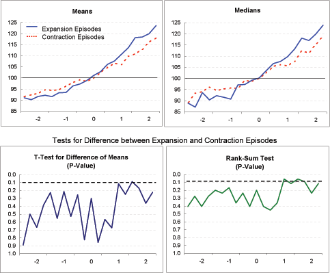
Data for Exhibit 4m

Year	Quarter	Means: Expansion	Means: Contraction	Medians: Expansion	Medians: Contraction	T-Test for Difference of Means	Rank-Sum Test
-2	1	91.0	91.6	88.9	89.3	0.89	0.40
-2	2	90.2	92.4	87.2	93.3	0.50	0.28
-2	3	91.7	93.0	93.6	94.1	0.67	0.40
-2	4	92.2	94.7	90.4	96.1	0.38	0.28
-1	1	91.6	94.4	92.3	94.6	0.23	0.20
-1	2	93.4	94.6	91.6	95.2	0.55	0.24
-1	3	93.4	96.4	90.7	95.7	0.22	0.17
-1	4	96.4	97.8	97.1	95.5	0.53	0.36
0	1	97.2	99.2	97.3	99.0	0.26	0.24
0	2	98.8	98.5	99.2	98.7	0.82	0.40
0	3	101.1	99.8	100.2	100.0	0.30	0.20
0	4	102.8	102.5	103.5	102.4	0.86	0.40
1	1	106.2	104.8	106.7	105.4	0.57	0.45
1	2	107.6	106.6	107.6	106.1	0.67	0.36
1	3	110.6	106.1	109.7	105.6	0.12	0.06
1	4	113.6	109.7	113.2	107.7	0.25	0.11
2	1	118.2	110.9	118.1	112.3	0.09	0.06
2	2	118.5	112.9	117.0	111.4	0.17	0.09
2	3	119.9	116.2	119.9	115.4	0.36	0.24
2	4	123.6	118.1	123.8	118.9	0.22	0.11

Exhibit 4n:  Real Import Index
Year 0 = 100

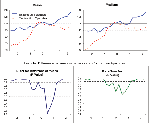
Data for Exhibit 4n

Year	Quarter	Means: Expansion	Means: Contraction	Medians: Expansion	Medians: Contraction	T-Test for Difference of Means	Rank-Sum Test
-2	1	94.7	83.1	94.6	80.7	0.07	0.02
-2	2	94.7	84.5	94.2	81.3	0.06	0.03
-2	3	96.5	84.1	94.7	84.3	0.01	0.01
-2	4	96.7	86.7	96.6	86.6	0.01	0.00
-1	1	95.5	87.0	93.6	87.8	0.02	0.01
-1	2	95.8	87.7	94.3	89.6	0.01	0.01
-1	3	98.1	90.9	96.7	90.8	0.01	0.00
-1	4	96.9	95.0	97.3	96.4	0.30	0.17
0	1	98.2	99.4	98.0	99.4	0.31	0.20
0	2	100.0	101.4	100.1	100.9	0.10	0.11
0	3	101.2	100.4	100.8	100.9	0.29	0.36
0	4	100.6	98.8	101.7	99.0	0.27	0.17
1	1	99.0	98.9	99.9	100.9	0.98	0.45
1	2	99.3	98.3	99.2	94.4	0.78	0.36
1	3	100.3	98.5	100.2	97.3	0.56	0.24
1	4	102.6	96.6	104.8	97.6	0.13	0.04
2	1	103.8	96.6	104.8	95.2	0.06	0.06
2	2	104.9	95.5	105.4	95.4	0.01	0.01
2	3	105.4	95.9	106.1	96.0	0.01	0.01
2	4	108.3	97.7	108.4	97.4	0.01	0.01

Exhibit 4o:  Nominal Imports / Nominal Exports Ratio

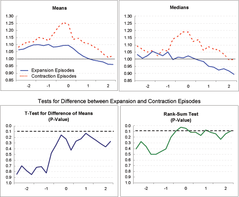
Data for Exhibit 4o

Year	Quarter	Means: Expansion	Means: Contraction	Medians: Expansion	Medians: Contraction	T-Test for Difference of Means	Rank-Sum Test
-2	1	1.06	1.08	1.03	1.09	0.85	0.40
-2	2	1.07	1.11	1.01	1.07	0.70	0.28
-2	3	1.09	1.12	1.02	1.05	0.78	0.36
-2	4	1.10	1.12	1.05	1.06	0.85	0.50
-1	1	1.10	1.15	1.04	1.03	0.72	0.50
-1	2	1.09	1.14	1.02	1.07	0.71	0.45
-1	3	1.10	1.13	1.05	1.06	0.82	0.40
-1	4	1.08	1.18	1.00	1.14	0.48	0.20
0	1	1.09	1.22	1.01	1.16	0.33	0.09
0	2	1.09	1.26	1.01	1.19	0.16	0.02
0	3	1.10	1.24	1.02	1.19	0.23	0.04
0	4	1.07	1.14	1.01	1.12	0.42	0.11
1	1	1.04	1.14	0.99	1.14	0.27	0.11
1	2	1.02	1.12	0.98	1.06	0.23	0.17
1	3	1.00	1.11	0.95	1.09	0.13	0.07
1	4	0.99	1.09	0.94	1.07	0.19	0.11
2	1	0.98	1.07	0.92	1.07	0.25	0.14
2	2	0.98	1.04	0.93	1.03	0.31	0.24
2	3	0.96	1.01	0.92	1.00	0.37	0.14
2	4	0.96	1.02	0.89	1.00	0.27	0.09

Exhibit 4p:  Budget Balance / GDP

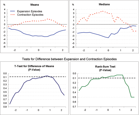
Data for Exhibit 4p

Year	Quarter	Means: Expansion	Means: Contraction	Medians: Expansion	Medians: Contraction	T-Test for Difference of Means	Rank-Sum Test
-2	1	-1.0	-0.5	-2.3	0.2	0.82	0.36
-2	2	-1.3	-0.4	-2.2	1.3	0.66	0.28
-2	3	-1.4	0.0	-2.1	1.9	0.53	0.28
-2	4	-1.5	-0.1	-2.2	0.9	0.50	0.24
-1	1	-1.9	0.2	-2.1	2.6	0.40	0.14
-1	2	-2.4	0.6	-2.3	2.7	0.25	0.11
-1	3	-2.7	0.8	-2.5	3.1	0.20	0.11
-1	4	-2.8	0.8	-2.8	3.1	0.18	0.11
0	1	-3.1	1.0	-3.0	3.6	0.13	0.07
0	2	-3.0	0.9	-3.3	3.3	0.14	0.09
0	3	-3.1	0.9	-3.5	3.0	0.12	0.07
0	4	-3.1	1.0	-2.4	2.8	0.11	0.06
1	1	-3.3	1.1	-2.6	0.6	0.08	0.06
1	2	-3.2	1.5	-2.2	2.1	0.06	0.03
1	3	-2.9	1.3	-0.9	1.4	0.09	0.03
1	4	-2.7	0.9	-1.1	0.6	0.11	0.03
2	1	-2.2	0.4	-1.0	0.3	0.22	0.20
2	2	-1.9	0.1	-0.5	-0.2	0.31	0.28
2	3	-1.6	-0.4	-0.3	-1.7	0.49	0.50
2	4	-1.5	-0.6	-0.4	-1.7	0.59	0.50

Exhibit 4q:  Structural Budget Balance / Potential GDP

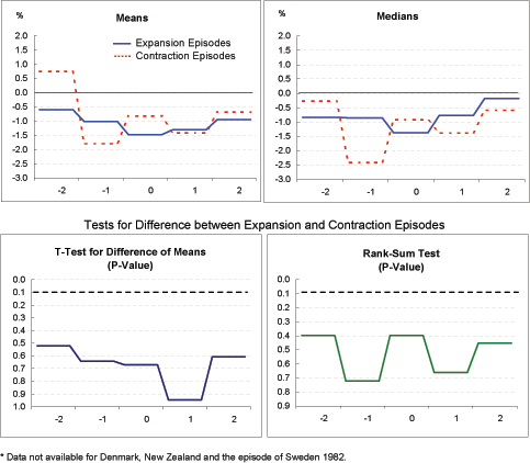
Data for Exhibit 4q

Year	Quarter	Means: Expansion	Means: Contraction	Medians: Expansion	Medians: Contraction	T-Test for Difference of Means	Rank-Sum Test
-2	1	-0.6	0.8	-0.8	-0.3	0.52	0.40
-2	2	-0.6	0.8	-0.8	-0.3	0.52	0.40
-2	3	-0.6	0.8	-0.8	-0.3	0.52	0.40
-2	4	-0.6	0.8	-0.8	-0.3	0.52	0.40
-1	1	-1.0	-1.8	-0.9	-2.4	0.64	0.72
-1	2	-1.0	-1.8	-0.9	-2.4	0.64	0.72
-1	3	-1.0	-1.8	-0.9	-2.4	0.64	0.72
-1	4	-1.0	-1.8	-0.9	-2.4	0.64	0.72
0	1	-1.5	-0.8	-1.4	-0.9	0.67	0.40
0	2	-1.5	-0.8	-1.4	-0.9	0.67	0.40
0	3	-1.5	-0.8	-1.4	-0.9	0.67	0.40
0	4	-1.5	-0.8	-1.4	-0.9	0.67	0.40
1	1	-1.3	-1.4	-0.8	-1.4	0.95	0.66
1	2	-1.3	-1.4	-0.8	-1.4	0.95	0.66
1	3	-1.3	-1.4	-0.8	-1.4	0.95	0.66
1	4	-1.3	-1.4	-0.8	-1.4	0.95	0.66
2	1	-0.9	-0.7	-0.2	-0.6	0.61	0.45
2	2	-0.9	-0.7	-0.2	-0.6	0.61	0.45
2	3	-0.9	-0.7	-0.2	-0.6	0.61	0.45
2	4	-0.9	-0.7	-0.2	-0.6	0.61	0.45

Exhibit 4r:  Net International Investment Position / Potential GDP

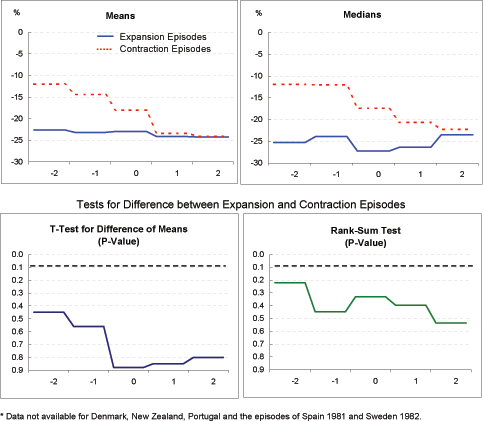
Data for Exhibit 4r

Year	Quarter	Means: Expansion	Means: Contraction	Medians: Expansion	Medians: Contraction	T-Test for Difference of Means	Rank-Sum Test
-2	1	-22.6	-12.0	-25.3	-11.9	0.45	0.22
-2	2	-22.6	-12.0	-25.3	-11.9	0.45	0.22
-2	3	-22.6	-12.0	-25.3	-11.9	0.45	0.22
-2	4	-22.6	-12.0	-25.3	-11.9	0.45	0.22
-1	1	-23.2	-14.4	-23.9	-12.0	0.56	0.45
-1	2	-23.2	-14.4	-23.9	-12.0	0.56	0.45
-1	3	-23.2	-14.4	-23.9	-12.0	0.56	0.45
-1	4	-23.2	-14.4	-23.9	-12.0	0.56	0.45
0	1	-22.9	-18.0	-27.3	-17.4	0.88	0.33
0	2	-22.9	-18.0	-27.3	-17.4	0.88	0.33
0	3	-22.9	-18.0	-27.3	-17.4	0.88	0.33
0	4	-22.9	-18.0	-27.3	-17.4	0.88	0.33
1	1	-24.1	-23.4	-26.4	-20.7	0.85	0.40
1	2	-24.1	-23.4	-26.4	-20.7	0.85	0.40
1	3	-24.1	-23.4	-26.4	-20.7	0.85	0.40
1	4	-24.1	-23.4	-26.4	-20.7	0.85	0.40
2	1	-24.2	-24.1	-23.5	-22.3	0.80	0.54
2	2	-24.2	-24.1	-23.5	-22.3	0.80	0.54
2	3	-24.2	-24.1	-23.5	-22.3	0.80	0.54
2	4	-24.2	-24.1	-23.5	-22.3	0.80	0.54

Exhibit 5:  Correlations Among Indicators Across All Episodes
(Indicators measured as changes from before to after current account troughs)

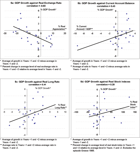
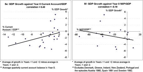
Exhibit 6:  Alternative Sorting Formula: Change in 3-year Averages of GDP 4-quarter Growth Rates

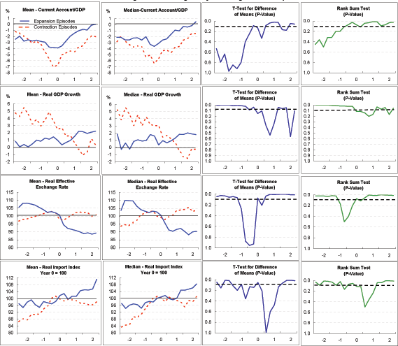
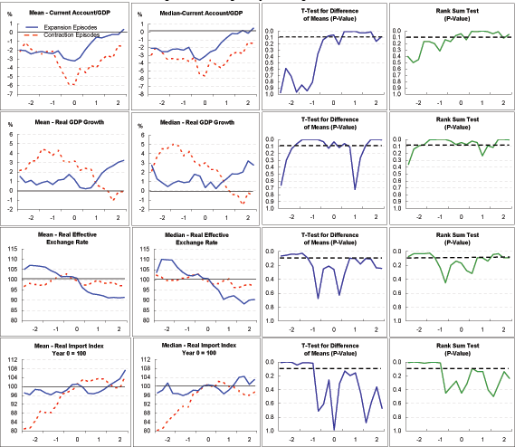
Footnotes

*   We would like to thank Caroline Freund, Joe Gagnon, Edward Gramlich, Luca Guerrieri, William Helkie, David Howard, Karen Johnson, Nathan Sheets, and participants in the International Finance Division workshop, as well as Benn Steil and two anonymous referees, for helpful comments. The views expressed in this paper are solely the responsibility of the authors and should not be interpreted as reflecting the views of the Board of Governors of the Federal Reserve System or of any other person associated with the Federal Reserve System. Return to text

**  Corresponding Author: Steven Kamin, Telephone 202-452-3339, Fax 202-872-4926. Email addresses: [email protected], [email protected], and [email protected]. Return to text

1.  See, among others, The Economist (2004), Eichengreen (2004), Hatzius (2004), Mann (1999, 2002), Mussa (2004), Obstfeld and Rogoff (2004), Ragan (2004), Roubini and Setzer (2004), Truman (2004), and Wolf (2004). Return to text

2.  Additionally, Obstfeld and Rogoff (2004) suggest that a future external adjustment in the United States might more closely resemble the experience of the 1970s than of the 1980s. Eichengreen (2004) argues that adjustment would likely induce a recession, both in the United States and abroad. Return to text

3.  See, for example, Hatzius (2004), Mussa (2004), Tilton (2004), and Truman (2004). Return to text

4.  Neither of these two cases makes clear why a run on dollar assets might also lead to a run on non-dollar assets, as posited in the more extreme versions of the disorderly correction scenario. Possibly, an abrupt decline in the dollar may lead to a rise in global risk premia, thus depressing all financial markets. Return to text

5.  In countries with substantial net foreign-currency denominated debt, a depreciation raises the domestic-currency value of this debt, inducing a reduction in net worth. This process is believed to have contributed to the sharp declines in domestic spending observed during many emerging market crises. However, U.S. balance sheets are believed to be much less exposed to a fall in the dollar, as the preponderance of U.S. debt is denominated in dollars. Return to text

6.  While Freund's study concentrates on the experience of industrialized economies, Milesi-Ferretti and Razin (2000) and Edwards (2004), among others, consider the current account adjustment process in low- and middle-income countries. The Bank for International Settlements' 2004 annual report also looks at financial flows along the adjustment process. The International Monetary Fund September 2002 World Economic Outlook extends Freund's study by particularly investigating the experience of countries with large current account deficits. Return to text

7.  See Milesi-Ferretti and Razin (2000) and Edwards (2004). Return to text

8.  This literature dates back at least to Diaz-Alejandro (1963). See, among many others, Krugman and Taylor (1978), Lizondo and Montiel (1989), and Calvo and Reinhart (2001). Return to text

9.  See Ahmed, Gust, Huntley, and Kamin (2002). Return to text

10.  In order to focus closely on the case of adjustment in industrialized economies, we dropped from our dataset cases of adjustment in Hong Kong, Israel, Korea, and Singapore that had been included in the Freund study. Return to text

11.  The new episodes were Greece, 1990, and Austria, 1999; the year of Portugal's adjustment was shifted from 1981 to 1982, and Belgium's was shifted from 1981 to 1980. We have confirmed that had we not incorporated these changes into our analysis, the basic findings described in this paper would have been little changed. Return to text

12.  The test is a modification of the Wilcoxon-Mann-Whitney test, called a robust rank-order test developed by Fligner and Pollicello (1981). The difference between the two approaches is that the Wilcoxon-Mann-Whitney assumes that the two samples have the same higher-order moments, whereas the robust rank-order test does not. Return to text

13.  As a result of the change in sorting mechanism, the US (1987) is replaced by Greece (1985) for the expansion episodes and Australia (1989) is replaced by Italy (1981) for the contraction episodes. Return to text

14.  To be clear, instead of calculating the growth rate of GDP for, say, 1987 as the growth from 1986 Q4 to 1987 Q4, we calculate it in the alternative procedure as the growth from the average level in 1986 to the average level in 1987. Based on this approach, US (1987) is replaced by Canada (1981) for the expansion episodes, and Denmark (1986), Portugal (1982), and New Zealand (1984) are replaced by Austria (1980), Austria (1999), and Greece (1985) for the contraction episodes. Return to text

This version is optimized for use by screen readers. Descriptions for all mathematical expressions are provided in LaTex format. A printable pdf version is available. Return to text

Home | Economic research and data | Publications and education resources
Accessibility | Contact us
Last update: August 20, 2008