
Board of Governors of the Federal Reserve System
International Finance Discussion Papers
Number 847, November 2005--- Screen Reader
Version*
The Baby Boom: Predictability in House Prices and Interest Rates
NOTE: International Finance Discussion Papers are preliminary materials circulated to stimulate discussion and critical comment. References in publications to International Finance Discussion Papers (other than an acknowledgment that the writer has had access to unpublished material) should be cleared with the author or authors. Recent IFDPs are available on the Web at http://www.federalreserve.gov/pubs/ifdp/. This paper can be downloaded without charge from the Social Science Research Network electronic library at http://www.ssrn.com/.
Abstract:
This paper explores the baby boom's impact on U.S. house prices and interest rates in the post-war 20th century and beyond. Using a simple Lucas asset pricing model, I quantitatively account for the increase in real house prices, the path of real interest rates, and the timing of low-frequency fluctuations in real house prices. The model predicts that the primary force underlying the evolution of real house prices is the systematic and predictable changes in the working age population driven by the baby boom. The model is calibrated to U.S. data and tested on international data. One surprising success of the model is its ability to predict the boom and bust in Japanese real estate markets around 1974 and 1990.
Keywords: Asset pricing, yield curve, great moderation
JEL classification: E21, E31, G12, R21
1 Introduction
This paper explores the extent to which the baby boom has impacted U.S. house prices and interest rates over the latter half of the 20th century. Without question, the baby boom has had a direct and large impact on the dynamics of the U.S. age profile. These dynamics have manifested themselves in changes to the proportion of the population that is of working age. The boomers entered the labor force en masse between 1967 and 1973 and, over the subsequent 35 years, they increased both the size and the growth rate of the potential labor force. The baby boomers are now about to leave the workforce. As they retire, the size of the working age population will fall as will output per person.
These changes in the working age population and the associated impact on output have had and will continue to have a first order effect on house prices and interest rates in the United States. This paper builds on the intuition of the well known paper by Mankiw and Weil (1988). That paper predicted that the baby boom would lead to a peak in house prices in 1989 (they were right) and then to a large permanent fall in the real price of housing from that point forward (obviously wrong). The intuition for this result is simple. If households exhibit hump-shaped demand for housing over the life-cycle and if housing is relatively difficult to build, then house prices should exhibit a peak at the time that the baby boomers reach their peak demand and should decline as the boomer's demand for housing wanes. The obvious gulf between their predictions and the increases in house prices between 1995 and the present have caused many to dismiss both the Mankiw and Weil paper and the impact of the baby boom on house prices in toto.
This paper will resurrect their intuition. Mankiw and Weil missed the upturn only because they worked in a partial equilibrium environment and over the course of the 1990s general equilibrium effects began to dominate the contemporaneous demand effects. In other words, they neglected both the impact of discount rates on house prices and the impact of the baby boom on the discount rate. By working in a structural model, this paper is able to consider the general equilibrium effects without neglecting the demand effects which are so important in the work of Mankiw and Weil. Indeed, I will show that, if the interest rate effect is shut down in my model, the model will replicate the predictions of Mankiw and Weil.
In this paper, the baby boom impacts house prices through demand effects which are very similar to those hypothesized by Mankiw and Weil; demand for housing is high when the working age population is large relative to the total population. However, this paper achieves a very different price path than that of Mankiw and Weil because the baby boom also affected interest rates and interest rates impact house prices.
In order to gain a quantitative idea of the magnitude of the effect of the baby boom on house prices, I develop a general equilibrium model which takes as input an exogenous demographic structure. Using a parsimonious and standard Lucas asset pricing framework, the model demonstrates that the demographic profile in the United States is a likely driver of both house prices and interest rates in the post-war era. In this paper, changes in the size of the working age population determine the labor input into a neoclassical production function. The model takes as given the endowment of capital, labor, and the stock of housing. As I work in an endowment economy, the model will not replicate the time series of capital accumulation - neither business nor residential. Since both of these stocks are assumed fixed, the model also misses the increase in consumption of both goods and housing services observed in the data. However, the model exactly replicates the increase in the ratio of consumption of goods and services to the consumption of housing services as reported in the National Income and Product Accounts. That is, the ratio of consumption to housing services increases by 18 percent in both the model and in the NIPA data over the period 1974 to 2004.1
When the size of the working age population is temporarily high as it is now, output is temporarily high and households wish to transfer assets to the future. Because ability to do so is limited2, there is upward pressure on real asset prices - house prices rise, interest rates fall.3 The increase in house prices occurs now despite the certain knowledge that once the baby boomers retire real house prices will fall.
The model is calibrated to replicate low-frequency U.S. house price movements between 1963 and 2005. Only two parameters of the model are used in the calibration - the elasticity of intertemporal substitution and the elasticity of intratemporal substitution. The first objective of the calibration is to exactly match the increase in house prices over the period 1963 to 2005. The second objective is to match the low-frequency swings in house prices. House prices have exhibited several cycles over the past 45 years and the goal of this paper is to replicate the timing and amplitude of these cycles using only demographics as an exogenous input to the model. The model is very successful at matching the timing of the housing cycle. With the exception of the 1973 peak in house prices, the model matches every peak in the data as well as every trough. While the model does quite well in matching the overall increase in house prices over time, it does not replicate the amplitude of the peaks and troughs.4 This model is the first model to my knowledge that is capable of matching each of the turning points in the data using a unified explanation.5
Without changing the parameters of the model, I test the model's ability to replicate the pattern of long-term real interest rates.6 Ignoring high frequency movement in the real rate, the model is consistent with interest rates over the period 1950 to 1972 during which interest rates rose and then fell and over the period 1990 to 2005 during which interest rates fell. In the intervening period, the model interest rate is too high relative to the data in the 1970s and too low relative to the data in the early 1980s. To restate this result, using the parameters which are designed to replicate house prices, the model exactly matches long-term interest rates for 37 of the past 55 years.
While the model misses the measured level of real rates in the 1970s, there are some interesting aspects of the nominal yield curve, in this time period, which are echoed in the real yield curve in the model. During this period, the nominal yield curve is consistently upward sloping. The common interpretation of this result is that agents had embodied large inflation expectations into the yield curve throughout the Fisher effect (Piazzesi and Schneider (2005)). In this model, the real yield curve is upward sloping. In the early 1970s, short rates are declining and long rates are increasing as they incorporate the increases in output which occur over the next 35 years.
The question remains "How rational do agents have to be in order to incorporate the output increases observed in the 1990s into the price of bonds being traded in the 1970s?" Do the agents need to have a demographic model like the one presented in this paper in order to anticipate the change in output? The answer is no. Individual agents simply looks forward to their own path of lifetime labor income. The agents in the model know their life time working hours and realize that their highest output years are yet to come. They realize that in the future their own household output per person will rise (their children becoming adults). Therefore, each agent wishes to borrow against these future increases in wealth. Unfortunately for them, the shock that they face turns out to be aggregate - their cohort goes to the bond market with them and interest rates rise. This is simply the flip side of why interest rates are low now.
One of the most surprising results of this paper is its ability to replicate the decline in output volatility in 1984. The volatility in output implied by our model falls by half in the post-1984 world. McConnell et al. (1999) identify a decline in the volatility of U.S. real GDP in 1984. This decline has been attributed alternatively to improved monetary policy (Clarida et al (2000)), improved business practices (McConnell et al. (1999), improved mortgage markets associated with regulation Q (Dynan et al (2005), or simply to a reduction in the volatility of macroeconomic shocks (Stock and Watson (2003)). The demographic model has none of these channels, implying that the good luck noted by Ahmed et al (2002) can simply be named predictable demographic changes. As the baby boom moderated so did the economy.
While it is a success in itself to match both house prices and interest rates in a such a parsimonious model, we further test the model's ability to match house prices in other industrialized countries. I test the model on data for the United Kingdom, Japan, and Ireland. The model succeeds in each case in matching both the trend in house prices and most of the major peaks in each country. Japan is the most remarkable case.
Between 1970 and 2005, Japanese real house prices exhibited peaks in 1974 and 1990. Since 1990, real house prices have fallen around 34 percent. The sharp increase in real estate prices in the 1980s followed by a fifteen-plus year fall in prices has led many to refer to 1980s Japan as the original bubble economy (Bayoumi and Collyns (2003)). This simple model, using Japanese demographic data, successfully predicts the 1974 and the 1990 house price peaks. Strikingly, the model also predicts a 30 percent decline in real house prices over the fifteen years following the 1990 peak.
The paper proceeds as follows. In the next section, I outline previous work on the link between asset prices and demographics. In section 3, the economy is presented and the two key asset pricing equations are derived. Section 4 outlines the key theoretical properties of the model. This section derives the link between interest rates and house prices. In section 5, the price responses of the model are simulated in order to give a quantitative feel for the theoretical results given in section 4. Section 6 inputs the baby boom into the model and calibrates the model to U.S. house prices. Section 7 gives the results of the calibrated model. Section 8 test the model on international data. Finally, I conclude.
2 Relationship to Previous Work
2.1 Baby Boom and Asset Prices
A number of previous studies have attempted to uncover the relationship, if it exists, between asset prices and the baby boom. These papers have met with only limited success. Almost all of these papers have focused on equity prices7 and almost without exception these papers have attempted to exploit life-cycle properties of savings and investment behavior. My primary concern with exploiting the life-cycle properties observed in the data is that it is not known a priori whether these changes are fundamental or whether they themselves are induced by the out-of-equilibrium dynamics. Indeed it might be argued that even institutional structures such as the social pension schemes have been maintained only because the baby boom has kept their cost relatively low. A different population age-profile would potentially have very different impacts on asset prices and hence would produce very different cohort behavior. It is with this concern in mind that I shut down such effects in the model.
Porterba (2004) offers a survey of many of these models. Abel (2001, 2003) shows in an over-lapping generations model that a baby boom followed by a baby bust reduces the life-time rate of return for the baby boom cohort. The results are sensitive to the specification of the bequest motive, which implies the results are quite sensitive to the specification of the life-cycle properties of consumption.8 Yoo (1994) incorporates the baby boom into a model of international capital flows. Brooks (2002) develops a general equilibrium overlapping generations model in which the return to capital and the return to bonds varies over the baby boom. Porterba (2001, 2003, 2004) finds little evidence of a robust empirical relationship between asset returns and the baby boom. Rios-Rull (2001) finds that the implications of the baby boom on asset prices is quite sensitive to the assumed steady state properties of the model. Storesletten (2003) offers a model similar in spirit to that of Yoo. In his model, Storesletten finds that changing immigration policy can offset the impact of the baby boom.
3 The Economy
The economy consists of a single representative agent. While more complicated demographics could easily have been implemented in the model, this framework ensures the absence of the life-cycle type savings behavior which is the focus of so much of the previous work. That is, the dynamics in this model are not driven by dissaving on the part of some sub-set of agents but rather by aggregate fluctuations in output. The representative agent framework will also allow closed-form solutions for the pricing equations. The closed-form solutions, in turn, give very clean theoretical results.
The baby boom will be modeled as changes in the agent's endowment of time. The amount of time that the agent has to work in any period represents the percentage of the population which is of working age in a period. In other words, changes in the size of the working age population relative to the total population are modeled by adjusting the endowment of time between 0 and 1. A value of 1 implies that the entire population is of working age; likewise, a value of zero implies the population is non-productive.9 Empirically, values for this number have varied between near 0.78 in 1972 to around 0.95 in 2005 for the United States. As the percent of the working age population exactly determines output in this economy, variation in the size of the working age population will map directly into changes in endowment of the consumption good.
One aspect of the economy which is significant and which the current exercise forgoes is endogenous capital accumulation. This omission is important as allowing households the ability to smooth consumption over time mitigates the effects of output declines. However, there are several reasons why this omission is not as restrictive as in many previous papers. The effects of capital accumulation on prices are not as straightforward in this model as in a standard model as capital interacts in a subtle manner with house prices. That is, accumulation of capital today increases output of market goods today which tends to raise house prices.
Further, I argue that most inter-generational savings is of second-order importance. The effects drawn upon here are not driven by transfers from young to old which have no effect on economy-wide consumption. Rather, the effects exploited in this paper are driven by the aggregate economy's inability to transfer consumption between today and tomorrow. In the model presented here, the shocks occur over 20 to 50 year time periods and are more-or-less uninsurable. The shocks have real effects beyond what would be mitigated by inter-generational transfers. Note, that independent of the level of the capital stock, upon the retirement of the baby boomers, labor input and therefore output fall.
The model also ignores international capital flows. That is, the model relies on a closed economy assumption. This assumption is important as differing demographic structures across the world may allow international risk sharing. However, although there are difference in the demographic structures across countries in the industrialized world these differences are actually quite small. Given the long-lived nature of the shocks and the similarity in shocks across countries risk sharing may not be possible. Risk sharing between the industrialized world and the developing world may be limited by the development of financial markets in the latter or by the omnipresent risk of sovereign default in much of the developing world.
3.1 Endowment
The agent is endowed with a fixed amount of time which may change from period-to-period; however, the time path for the labor endowment is known with probability one from time zero. That is, while the time endowment may shift over time, the agent has perfect foresight over these changes.
The agent is endowed with a unit of housing. This assumption is intended to mirror an assumption in the data section in which the stock of housing per person is held constant. The critical assumption is that the stock of housing is not a function of the time endowment of the agent.
3.2 Technology
The model is a simple two sector model. One sector produces consumption goods taking labor as input. Labor is transformed to efficiency units through a productivity parameter. The other sector (thought of as the home sector) takes the stock of housing capital, scales it by a productivity factor, and produces housing services. Production of housing services does not require time as an input. Output from neither sector is storable, although housing capital itself is thought of as perfectly durable. Productivity is assumed constant in both sectors.
3.3 The Agent's Problem
The representative agent chooses sequences of consumption,
![]() and housing capital,
and housing capital, ![]() and zero-net supply bonds,
and zero-net supply bonds, ![]() in
order to maximize a time additively separable utility function as
follows:
in
order to maximize a time additively separable utility function as
follows:
|
(1) | |
![]() is the time
is the time ![]() endowment of
time.
endowment of
time. ![]() is normalized to lie on the interval
between 0 and 1. The implicit price of the zero-net supply bonds is
is normalized to lie on the interval
between 0 and 1. The implicit price of the zero-net supply bonds is
![]() and the price of housing
capital is
and the price of housing
capital is ![]()
![]() and
and
![]() are productivity factors on housing
capital and labor respectively. The parameter
are productivity factors on housing
capital and labor respectively. The parameter ![]() may be thought of as a parameter which maps stocks
of housing into flows of housing services. Housing services,
may be thought of as a parameter which maps stocks
of housing into flows of housing services. Housing services,
![]() today are produced by the stock of
housing denoted
today are produced by the stock of
housing denoted ![]() This assumption is a timing
convention and is without loss of generality. The agent discounts
future utility at rate
This assumption is a timing
convention and is without loss of generality. The agent discounts
future utility at rate ![]()
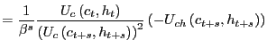
Prices adjust such that the following equilibrium conditions are satisfied
The equilibrium conditions make it clear that the agent may not transform market output to home output nor may the agent transform home output to market output. There is no storage.
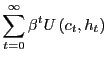
The first order conditions are as follows:
where
![]() is the Lagrange multiplier on the
time
is the Lagrange multiplier on the
time ![]() budget constraint. One may solve for
budget constraint. One may solve for
![]() by finding a solution to the difference
equation implied by the first order condition for
by finding a solution to the difference
equation implied by the first order condition for ![]() After substituting for
After substituting for
![]() from the first order condition
for
from the first order condition
for ![]() the solution is found by iterating
forward on
the solution is found by iterating
forward on ![]() as follows:
as follows:
|
||

|
||

|
||
|
(2) |
The first term in the last line,
![]() is simply the agent's effective rate of time discount between
period
is simply the agent's effective rate of time discount between
period ![]() and period
and period ![]() . This term
is often referred to as the pricing kernel and is the factor used
to discount the payoff of any future return.10 The second term
in the last line,
. This term
is often referred to as the pricing kernel and is the factor used
to discount the payoff of any future return.10 The second term
in the last line,
![]() can be thought of as the dividend payout from housing. The flow
value of housing is the marginal utility of housing evaluated at
the stock of housing scaled by the marginal utility of consuming
evaluated at the endowment of consumption. Housing is not special
in this model. The price of a consul bond with dividend flow equal
to
can be thought of as the dividend payout from housing. The flow
value of housing is the marginal utility of housing evaluated at
the stock of housing scaled by the marginal utility of consuming
evaluated at the endowment of consumption. Housing is not special
in this model. The price of a consul bond with dividend flow equal
to
![]() would perfectly commove with the price of housing.
would perfectly commove with the price of housing.
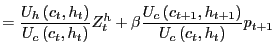
Interest rates evolve according to the following equation:
|
(3) |
where ![]() denotes the total rate of return
between period
denotes the total rate of return
between period ![]() and
and ![]() The
expectations hypothesis for the term structure of interest rates
holds exactly in this model, i.e. long real rates are simply the
product of one period returns.
The
expectations hypothesis for the term structure of interest rates
holds exactly in this model, i.e. long real rates are simply the
product of one period returns.
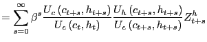
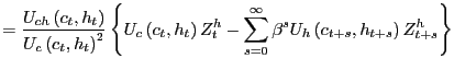
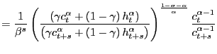
Combining the equation for house prices and the equation for interest rates, we derive the commonly used expression for the price of housing.
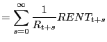 |
(4) | |
|
(5) |
The price of housing in period ![]() is the present
discounted value of rents, where the appropriate discount rate is
the real interest rate. This equation is often misused and is the
equation by which the statement "housing is under-responsive to
interest rates" (Campbell et al (2005)) is made. If we hold rents
constant, then this equation implies that prices must respond
one-for-one with any permanent change in interest rates. Think of
the example in which we simply reduce the entire term structure by
a factor
is the present
discounted value of rents, where the appropriate discount rate is
the real interest rate. This equation is often misused and is the
equation by which the statement "housing is under-responsive to
interest rates" (Campbell et al (2005)) is made. If we hold rents
constant, then this equation implies that prices must respond
one-for-one with any permanent change in interest rates. Think of
the example in which we simply reduce the entire term structure by
a factor ![]() Then
Then
|
(6) |
the price level simply adjusts by the factor
![]() Since measured real rates
appear extremely persistent (Campbell et al (2005)), any measured
change in the real rate would be expected to have a large effect on
the price level. The fact that this is not true in the data leads
to the under-responsive statement above. However, this thought
experiment is based on a false premise - that we can change
interest rates and not the flow of rents. In this class of models,
house prices and interest rates are driven by the same underlying
fundamentals - the time series of housing and goods consumption.
Changes in the path of either will, in general impact both assets.
In section 4 below, I show that only in the case where
Since measured real rates
appear extremely persistent (Campbell et al (2005)), any measured
change in the real rate would be expected to have a large effect on
the price level. The fact that this is not true in the data leads
to the under-responsive statement above. However, this thought
experiment is based on a false premise - that we can change
interest rates and not the flow of rents. In this class of models,
house prices and interest rates are driven by the same underlying
fundamentals - the time series of housing and goods consumption.
Changes in the path of either will, in general impact both assets.
In section 4 below, I show that only in the case where ![]() is zero can this experiment be reliably conducted.
is zero can this experiment be reliably conducted.
4 Theoretical Analysis
In this section, the relationship between prices interest rates and output at all horizons is established.11 Perhaps the most important result in this section is Corollary 2. Conventional wisdom based on equation 4 is that house prices and interest rates must have an inverse relationship. That is, any increase in the interest rate must lower house prices. This statement turns out to be parameter dependent. Because any change in interest rates is, in general, associated with a change in rents, this statement is only true if the cross derivative between housing and consumption is negative. This result is important because it shows us that the intuition which leads to equation 5 is fatally flawed.
The response of interest rates to a change in future consumption is straightforward and standard. Agents would like to smooth consumption. Because they are unable to do so, bond prices must adjust such that the agent is content with his current endowment.
Proposition 1 A fall in future
goods consumption at date ![]() decreases interest
rates for bonds paying off in period
decreases interest
rates for bonds paying off in period ![]() but leaves
other interest rates unchanged:
but leaves
other interest rates unchanged:
![]() with equality
if and only is
with equality
if and only is ![]()
Proof. This result is straight forward from the bond
pricing equation or from the fact that the expectations hypothesis
holds in this model. The payoff of a bond paying off in period
![]() is affected by changes in allocations in
those periods only. That is only for the period to which the agent
would like to reallocate consumption does the interest rate
structure change. This is immediate from the formula
is affected by changes in allocations in
those periods only. That is only for the period to which the agent
would like to reallocate consumption does the interest rate
structure change. This is immediate from the formula
![]()
A direct implication of the above theorem is that changes in future consumption move the term structure of interest rates in a very specific manner. The following corollary shows that the yield curve becomes generally flatter only for changes in consumption which occur over long periods of time. That is, short term changes in consumption impact interest rates at specific horizons; therefore, a flatter yield curve consumption implies lower consumption at all long dates relative to all short dates.
Corollary 1 The yield curve
becomes flatter (steeper) between bonds dated ![]() and bonds dated
and bonds dated ![]() if consumption falls (increases)
at all dates
if consumption falls (increases)
at all dates ![]() :
:
![]()
![]() .
.
Proof. The result follows from the above theorem.
Since
![]() with equality
if and only if
with equality
if and only if
![]() then
then
![]() if and only if
if and only if
![]()
Whereas the impact of changes in consumption on interest rates
is immediate, the sign of the change in house prices today in
response to a future fall in consumption is ambiguous. The reason
for the ambiguity is because housing is a durable good and hence
its price is impacted by the discount rate but it is also a
consumption good and hence its price is impacted by its relative
scarcity. Take the case of a fall in future consumption. The fall
in consumption lowers interest rates which puts upwards pressure on
house prices. However, the fall in consumption also makes housing
relatively plentiful which puts downward pressure on prices. The
relative strength of these two forces determines whether prices
rise or fall in response to changes in future consumption. As the
next proposition shows, the relative strength of the two affects is
determined by the sign of the cross-derivative, ![]()
Proposition 2 The real price of
housing rises (falls) in response to a fall (rise) in future goods
consumption if and only if the cross-derivative between consumption
of goods and the consumption of housing is negative:
![]()
Proof. This result is straightforward from
differentiation of the pricing equation for housing. We have after
simplifying
![]() Differentiating with respect to
Differentiating with respect to ![]() , we have
, we have
![]()
The last result occurs because there is a direct and an indirect
effect. Consumption falls so we wish to move consumption to that
period on the other hand the relative price of consumption in that
period rises so we would like to move more consumption to that
period in the form of housing. Our ability to make this trade-off
then relies on relative elasticities. The same effect can be seen
in examining the response of interest rates to changes in
![]() In this case, the interest rate
effect also depends on the relative elasticities or more
specifically on the sign of the cross-derivative.
In this case, the interest rate
effect also depends on the relative elasticities or more
specifically on the sign of the cross-derivative.
Proposition 3 Interest rates rise
(fall) in response to a rise (fall) in future housing consumption
if and only if the cross-derivative between consumption of goods
and the consumption of housing services is negative:
![]()
Proof. Again the equation for interest rates is
|
||
 |
|
Since the first two terms of the derivative are always positive,
![]()
![]()
It has long been assumed in the empirical and theoretical
literature that housing and interest rates should have an inverse
relationship. The last two theorems show that this does not have to
be the case. Indeed the previous propositions show that the change
in interest rates and prices will depend on the both the sign of
![]() and on whether interest rates and
house prices are responding to future or contemporaneous movements
and whether the movements are caused by changes in
and on whether interest rates and
house prices are responding to future or contemporaneous movements
and whether the movements are caused by changes in ![]() or
or ![]() .
.
Corollary 2 House prices and
interest rates have a weak inverse relationship if and only if the
cross-derivative between consumption of good and the consumption of
housing is negative: sign
![]()
![]()
Proof. The result is checked first for ![]() and then for
and then for ![]() If
If ![]() , above it was shown that
, above it was shown that
![]() but
but
![]() . Hence, for the case of changes in future consumption the result
is shown. If
. Hence, for the case of changes in future consumption the result
is shown. If ![]()
![]() but
but
![]() Given the if and only if relation for both
Given the if and only if relation for both ![]() and
and
![]() the proof is complete.
the proof is complete.
At this point, the relationship between both interest rates and prices to changes in future consumption of housing and market goods has been established. The response of house prices to contemporaneous changes in consumption is now examined.
Condition 1
![]()
Condition 1 is a statement on the relative scarcity of consumption of numeraire relative to housing consumption. If the condition holds, housing is sufficiently scarce that consuming one extra unit of housing forever is worth more than consuming an extra unit of consumption today.
Proof.
Proposition 4 House prices rise
(fall) in response to a contemporaneous rise (fall) in consumption
if and only if the cross-derivative between housing and consumption
is negative:
![]()
Proof. Using the price of housing
![]() and this time differentiating with respect to
and this time differentiating with respect to ![]() .
.
|
||
|
Hence
![]()
![]()
and a similar result for the response of interest rates to a contemporaneous change in housing
Proposition 5 Interest rates at
any horizon ![]() rise (fall) in response to a
contemporaneous rise (fall) in housing consumption if and only if
the cross-derivative between consumption of goods and the
consumption of housing is positive:
rise (fall) in response to a
contemporaneous rise (fall) in housing consumption if and only if
the cross-derivative between consumption of goods and the
consumption of housing is positive:
![]()
Proof. Using the interest rate equation for an
arbitrary horizon ![]()
![]() and differentiating with respect to
and differentiating with respect to ![]() , implies
, implies
![]() once again implying
once again implying
![]()
Implications of the model are now examined.
5 Simulation
In this section, we study the magnitude of the response in prices and interest rates to changes in the time path of consumption. The simple experiments given in this section will not only demonstrate how the theoretical results derived in the last section work in practice but will also pin down the potential magnitudes of changes in output on asset prices. That is, does the fact that house prices have the potential to increase in the face of a known future change in output have relevance or is the change so small as to be beneath recognition.
The two relevant pricing equations, in terms of the CES utility function, are
|
(7) | |
|
(8) |
The top equation is the price of housing and the bottom is the real
interest rate. In order to ease exposition, define the function
 Written in this manner, the discount of future payoffs changes
symmetrically (modulo
Written in this manner, the discount of future payoffs changes
symmetrically (modulo ![]() to changes in
to changes in
![]() and
and ![]() but
only change in
but
only change in ![]() affect future rents. This
formulation turns out to be convenient when examining the effect of
changes in consumption on prices.
affect future rents. This
formulation turns out to be convenient when examining the effect of
changes in consumption on prices.
The model has four parameters which must be chosen - ![]()
![]() The parameter
The parameter
![]() determines the share of housing
consumption in utility This parameter can be adjusted to match any
level of prices (see Davis and Martin 2005).12 The parameter
determines the share of housing
consumption in utility This parameter can be adjusted to match any
level of prices (see Davis and Martin 2005).12 The parameter
![]() is the standard time discount rate.
This parameter will be set such that the real interest rate is 4
percent over any constant consumption path. The parameters
is the standard time discount rate.
This parameter will be set such that the real interest rate is 4
percent over any constant consumption path. The parameters
![]() and
and ![]() govern
the elasticity of intratemporal substitution and the elasticity of
intertemporal substitution respectively. In terms of the
theoretical analysis section, it is these two parameters which
govern the sign of the cross-derivative,
govern
the elasticity of intratemporal substitution and the elasticity of
intertemporal substitution respectively. In terms of the
theoretical analysis section, it is these two parameters which
govern the sign of the cross-derivative, ![]()
As a reminder, for the CES utility function, the sign of the
cross-derivative depends entirely on the sign of
![]()
If the two types of goods are more substitutable intratemporally
than intertemporally, then
![]() and the
cross-derivative is positive, otherwise it is negative. Notice,
that, since
and the
cross-derivative is positive, otherwise it is negative. Notice,
that, since
![]() , the
cross-derivative is positive only if the two goods are
significantly more complementary than Cobb-Douglas utility
, the
cross-derivative is positive only if the two goods are
significantly more complementary than Cobb-Douglas utility
![]() .
.
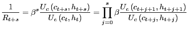
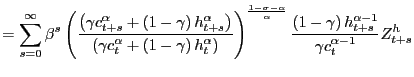
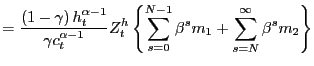
5.1 Permanent Fall in Consumption N Periods Ahead
In the first experiment, the impact of a permanent fall in
consumption ![]() periods in the future is examined. The
fall in consumption
periods in the future is examined. The
fall in consumption ![]() periods in the future is
revealed in period
periods in the future is
revealed in period ![]() .13 We can use summation
by parts to write the pricing equation for housing in two pieces as
follows:
.13 We can use summation
by parts to write the pricing equation for housing in two pieces as
follows:
|
(9) | |
|
The first term is the sum over all dates up to the event date and
the second term is the sum of all dates on or after the event date.
Since the above equation is the time ![]() pricing
equation, the denominator of both
pricing
equation, the denominator of both ![]() and
the rent term consist solely of date
and
the rent term consist solely of date ![]() values
implying that the denominator is the same before and after the
event date.
values
implying that the denominator is the same before and after the
event date.
Since consumption falls permanently at date ![]() and is unchanged between
and is unchanged between ![]() and
and ![]()
![]() takes on only two distinct values.
It takes on value
takes on only two distinct values.
It takes on value ![]() for all dates prior to
the event date and value
for all dates prior to
the event date and value ![]() for all dates on or
after the event date. Recalling that
for all dates on or
after the event date. Recalling that ![]() is constant
by assumption, the pricing equation can be written as follows
is constant
by assumption, the pricing equation can be written as follows
|
||
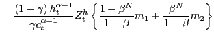
|
(10) |
where the second equation uses the formula for geometric sums to
arrive at a closed form solution for the time ![]() price of housing.
price of housing.
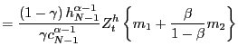
The formula for the price of housing is simply a weighted sum of
![]() and
and ![]() where the
relative weights are a function of the remaining time between the
current period,
where the
relative weights are a function of the remaining time between the
current period, ![]() , and the event date,
, and the event date, ![]() As the economy approaches the event date, the weight on
As the economy approaches the event date, the weight on
![]() converges from below to
converges from below to
![]() and the weight on
and the weight on
![]() converges from above to zero. That is,
the difference between consumption at date
converges from above to zero. That is,
the difference between consumption at date ![]() and
consumption after the event date becomes increasingly important as
the event date approaches.
and
consumption after the event date becomes increasingly important as
the event date approaches.
Whether prices rise or fall as the economy nears the event date
is determined by the relative size of ![]() and
and
![]() If
If ![]() is larger than
is larger than
![]() , house prices will fall as
, house prices will fall as ![]() approaches the event date,
approaches the event date, ![]() In this
example
In this
example ![]() is less than
is less than ![]() so
so
![]() will be larger than
will be larger than ![]() if the power
if the power
![]() is positive.
That is,
is positive.
That is, ![]() will be larger than
will be larger than ![]() if goods are more substitutable intertemporally than
intratemporally (Proposition 2).
if goods are more substitutable intertemporally than
intratemporally (Proposition 2).
Do house prices rise or fall between periods ![]() and
and ![]() The pricing equation at date
The pricing equation at date
![]() and
and ![]() are as follows
are as follows
|
||
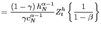
|
(11) |
Since
![]() and
and ![]() is positive,
is positive, ![]() is
always less than
is
always less than ![]() House prices fall
discreetly at the event date. This is true independent of
assumptions on parameters. Rents fall because housing is relatively
less scarce after the event date and house prices are just the
discounted sum of rents. By extension, house prices are also lower
after the event date than before the announcement date.
House prices fall
discreetly at the event date. This is true independent of
assumptions on parameters. Rents fall because housing is relatively
less scarce after the event date and house prices are just the
discounted sum of rents. By extension, house prices are also lower
after the event date than before the announcement date.
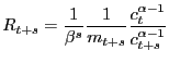
Figure 1 shows the price of housing for a specific
parameterization. Prior to the announcement date, period 1,
consumption of both housing and other goods are set equal to
one![]() At date
At date ![]() the announcement
that consumption of goods will fall by 30 percent at date 50 is
made. Figure 4 shows the evolution of house prices from five
periods before the announcement until ten periods after the event
date for several different values
the announcement
that consumption of goods will fall by 30 percent at date 50 is
made. Figure 4 shows the evolution of house prices from five
periods before the announcement until ten periods after the event
date for several different values ![]() . The
other parameters are set as follows: (
. The
other parameters are set as follows: (![]()
![]()
![]() The first vertical line
demarcates the announcement date and the second vertical line
demarcates the event date.
The first vertical line
demarcates the announcement date and the second vertical line
demarcates the event date.
Prices rise in response to the announcement and continue to rise
until the event date for all values of ![]() which
are greater than -2 (
which
are greater than -2 (![]() . When
. When ![]() is equal to -2, price do not change until the actual
event date when rents fall. For all values of
is equal to -2, price do not change until the actual
event date when rents fall. For all values of ![]() less than -2, price fall steadily between the
announcement date and the event date. In all cases, the price of
housing falls at the event date. The fall in price occurs because
at date 50 rents fall precipitously14 The important thing
to take away from this simulation is that the price of housing can
rise today even in the face of a perfectly certain fall in prices
in the future.
less than -2, price fall steadily between the
announcement date and the event date. In all cases, the price of
housing falls at the event date. The fall in price occurs because
at date 50 rents fall precipitously14 The important thing
to take away from this simulation is that the price of housing can
rise today even in the face of a perfectly certain fall in prices
in the future.
Housing, acting effectively as a consul bond paying off in
rents, is affected period-by-period between period ![]() and
and ![]() The interest rates on single period bonds
and the term structure are however only affected at intervals over
which the event occurs. Using our notation, the
The interest rates on single period bonds
and the term structure are however only affected at intervals over
which the event occurs. Using our notation, the ![]() period interest rate is written as follows
period interest rate is written as follows
|
(12) |
For dates ![]() and
and ![]() less than 50, the
interest rate at horizon
less than 50, the
interest rate at horizon ![]() is determined solely by
is determined solely by
![]() For interest rates
which cross the date
For interest rates
which cross the date ![]() and
and
![]() are both reduced.
After date 50, the interest rate at horizon
are both reduced.
After date 50, the interest rate at horizon ![]() is once
again governed by
is once
again governed by
![]() alone. Here the
flattening of the yield curve is actually a kink (because of the
discrete nature of the event). As we approach the event date, short
rates are unaffected and long rates are lower by the factor
alone. Here the
flattening of the yield curve is actually a kink (because of the
discrete nature of the event). As we approach the event date, short
rates are unaffected and long rates are lower by the factor
![]() .
When
.
When ![]() is 0.5, this factor is 0.45. That is
interest rates are only 45 percent as large as an equivalent
horizon interest rate which does not span the event date. When
is 0.5, this factor is 0.45. That is
interest rates are only 45 percent as large as an equivalent
horizon interest rate which does not span the event date. When
![]() is -0.5, the factor drops to -0.39.
By the time
is -0.5, the factor drops to -0.39.
By the time ![]() is -5, the factor has dropped to
0.28.15
is -5, the factor has dropped to
0.28.15
5.2 Changes in the Growth Rate of Consumption (a baby boom)
The second experiment is designed to show how house prices
behave along different consumption paths. To fix ideas, the value
of ![]() is set to -.05 and the value of
is set to -.05 and the value of
![]() is set to 3. This experiment is meant
to demonstrate the mechanisms at work over a baby boom. To do so,
consumption will be held constant for 25 years (pre-entry into
workforce), allowed to grow at 1 percent per year for 25 years (the
baby enters the workforce), held constant again for 25 years (not
yet retired), and then fall at 0.5 percent for 25 years (the baby
boom retires) before being held constant for the infinite future
(back to the steady state). Figure 1a shows the results of this
simulation. The solid line is the price path of housing. The dashed
line is the path of rents. Recall that the path of rents is
isomorphic to the path of consumption. The dashed dot line is the
rent-to-price ratio for this economy.
is set to 3. This experiment is meant
to demonstrate the mechanisms at work over a baby boom. To do so,
consumption will be held constant for 25 years (pre-entry into
workforce), allowed to grow at 1 percent per year for 25 years (the
baby enters the workforce), held constant again for 25 years (not
yet retired), and then fall at 0.5 percent for 25 years (the baby
boom retires) before being held constant for the infinite future
(back to the steady state). Figure 1a shows the results of this
simulation. The solid line is the price path of housing. The dashed
line is the path of rents. Recall that the path of rents is
isomorphic to the path of consumption. The dashed dot line is the
rent-to-price ratio for this economy.
First, note that house prices are not constant during either of the periods in which consumption is not changing. Not surprisingly given the results of the last simulation, the path of prices in influenced by future consumption. Over the first twenty five years, the agent looks forward to the relatively good times once the baby boom enters the workforce. The relatively high interest rates imply falling house prices over this period. In the second zero consumption growth period - periods 50 through 75 - prices rise as real interest rates fall in anticipation of the baby boom's retirement. Over the period with rising consumption, the increase in house prices is almost double the increase in rents. This rise occurs because consumption is rising relative to housing raising rents and because real interest rates are falling because consumption will grow less quickly in the future. The rent-to-price ratio reaches a high of just above 4.7 in period 25 before plummeting to a low of 3.7 in year 75. The rent-to-price ratio returns to its steady state value of 4 at the end of the sample as consumption remains constant from period 100 forward.
6 The U.S. Baby Boom
6.1 Interpreting the Baby Boom in a RA Model
The model will now be fit to the U.S. data. The model presented above is a representative agent model. In order to replicate the impact of the baby boom, the time endowment of the agent will be adjusted to match the proportion of the population which is of working age. That is, if half of the population is between the ages of 25 and 64, the time endowment of the representative agent will be 0.5. Notice that this assumption implies that agents who are working age are engaged in productive activity whether or not they are in the formal market sector. This view is not completely standard but is consistent with the home production literature and the human capital accumulation literature. That is if a person of working age is not in the traditional labor force then they are engaged in some type of home production (for example, a woman who quits work to raise children is producing home goods). The assumption assumes that retirees and children have zero productivity. At this time, no attempt is made to adjust these populations. For example, one might think that while the output of retirees relative to their consumption is lower than a working age person, that output is still positive. Similarly for children. Indeed Francis and Ramey (2005), attempt to include a subset of both of these populations in their measure of the potential labor force. A generalization of the model might wish to specifically consider this aspect.
6.2 Key Features of the U.S. Data
To begin, the model will be tested against data from the United
States. Figure 2 shows the total population, the working age
population, and the population under the age of five for the United
States from 1940 to 2099 (data from 2005 forward are
projections16). The original baby boom, the baby
bust, and the subsequent baby boomlet are evident in the data. The
growth rate of the population under five is high relative to the
rest of our sample from 1937 to nearly 196017. Figure 3 shows
the evolution of the age 5 and under population as a percent of the
total population from 1901 to 2003. Notice, over the 20![]() century the percent of the under-five population has
fallen from around 12 percent in 1901 to just under 7 percent in
2003. The dynamics of the under 5 population have direct
implications for the dynamics of the working age population (i.e. a
smaller under-five population in 1980 leads to fewer 25 year-olds
in 2005). This impact can be seen in figure 3.
century the percent of the under-five population has
fallen from around 12 percent in 1901 to just under 7 percent in
2003. The dynamics of the under 5 population have direct
implications for the dynamics of the working age population (i.e. a
smaller under-five population in 1980 leads to fewer 25 year-olds
in 2005). This impact can be seen in figure 3.
Figure 4 shows the evolution of the working age population as a percent of the total population from 1940 through 2099. As a result of the baby boom, the working age population begins to rapidly increase around 1970 and then begins to decrease around 2020. For one remarkable 30 year episode, the working age population in the United States grew at a rate much greater than its long-term average growth rate. Over approximately the next 30 years, the working age population relative to the total population is predicted to shrink.
There are several key features of this data which the model will attempt to match. First and foremost the model will attempt to replicate real house price data from 1963 through 2005. Real house prices for the United States are shown in Figure 5. The relative price of housing has doubled over the past 45 years. Over the same 45 year period, there have also been several substantial swings in house prices. The challenge for any house price model is to match both the substantial increase over the entire period and at the same time match the intermediate fluctuations in house prices. We will show the model presented above, when fed the time path of the U.S. working age population, is capable of reproducing both features of the data.
Second, the model will attempt to match the time series of long-term real interest rates for the United States. Real interest rates for the United States are shown in Figure 6. The solid bold line is the real ten-year Treasury rate. The dashed black line is the real one-year Treasury rate. These series are created by subtracting a measure of inflation expectations from the nominal rate. If the risk premium, that is the agent's view on the volatility of inflation are not constant, then these time series may differ significantly from the true real rate.
In particular, the data spans two relatively stable and low-inflation periods - 1950 to the late 1960s and the mid-1980s to the present - and a high and volatile inflation period - 1970 to the early 1980s. It is likely that inflation expectations are reasonably approximated and that the risk premium is fairly constant over the stable periods but for the 1970s there is no good method of determining the accuracy of the real rate. The fact that the measured real rates are quite negative does give one pause. Arguably inflation stabilized by the mid-to-early 1980s as a result of the Volcker disinflation. However, a recent paper by Goodfriend and King (2005) argues that inflation expectations remained quite high over this period. Hence, the true level of the real rate over the early 1980s is probably not well represented by my measure of real rates.
Nevertheless, I characterize the long rate as having two humps. The first hump runs from 1954 to 1977 and achieves a peak in 1966. The second hump covers the period 1978 to 2005 and peaks in 1984. I will completely ignore short-term fluctuations in the measured real rate. The model will be compared to the two-hump shape of the real rate.
It is worth noting how consumption in the model measures up to consumption in the data. In the model, one of the most important dynamics is the increase in consumption between 1973 and 2004. Over this time period, model consumption increases 18 percent. Since the stock of housing is assumed constant in this exercise, the consumption of goods relative to consumption of housing services increases the same amount. For U.S. data between 1973 and 2004, real consumption as measured by line 1 of table Table 2.3.3. from the National Income and Product Accounts increased by 98 percent, a bit more than consumption in the model. However, the growth rate of real consumption relative to real housing services, line 14 of table 2.3.3, also rose 18 percent. Since what matters most for the model is the relative growth rate of consumption this is very close. Therefore, ignoring relative productivity changes in the model seems to be well approximated by the data at least in the very long run. This allows the model to avoid taking a stand on the pattern of productivity growth in future years.
6.3 Fitting the Model to the Data
The only external input to the model is the relative size of the working age population. This data was shown in Figure 3. The baby boom has effected the relative size of the working age population since they were born. The size of the working age population declined steadily from 1945 to around 1973. Note that this decline ended 25 years after the beginning of the baby boom implying the decline is occurring as older cohorts are retiring and the boomers are not yet of working age. Since 1973, the percentage of the population of working age has increased fairly steadily. The influx of baby boomers into the workforce moved the ratio of working age population to total population from a low of around 79 percent in 1973 to nearly 96 percent in 2005. The ratio is projected to hit an all time high of 97 percent in the year 2017. In the model, these changes in the proportion of the working age population feed directly into the time series of labor input and hence feed directly into changes in consumption.
Recalling the relative forces on house prices from the simulation and theoretical analysis sections, contemporaneous increases (falls) in consumption increase (decrease) house prices. Future, changes in consumption may put upwards or downwards pressure on consumption depending on whether the inter or intratemporal elasticity of substitution is stronger. As a result, given the increase in the working age population over the sample period, matching the general increase of house prices is straightforward.
6.4 Matching the Average Increase and Mankiw and Weil
To illustrate the ease with which the average trend is house
prices is matched, the discount rate is set to zero leaving only
the parameters ![]() and
and ![]() to
match the average time series of house prices. The solid bold line
in Figure 7 gives the results of this exercise.
to
match the average time series of house prices. The solid bold line
in Figure 7 gives the results of this exercise. ![]() The object of the exercise is to match the average increase
in house prices over the time period. This will be true if the
endpoints of the simulated and actual series match. In other words,
the model is to match two data points using two degrees of freedom.
For convenience, set
The object of the exercise is to match the average increase
in house prices over the time period. This will be true if the
endpoints of the simulated and actual series match. In other words,
the model is to match two data points using two degrees of freedom.
For convenience, set ![]() such that the price
series match in 1963 and then change
such that the price
series match in 1963 and then change ![]() until
they also match in 2005. The average increase between 1963 and 2004
is exactly replicated. In this case, the price of housing is also
simply a monotone transformation of the working age population.
until
they also match in 2005. The average increase between 1963 and 2004
is exactly replicated. In this case, the price of housing is also
simply a monotone transformation of the working age population.
One note of interest is that in this example, the results of
Mankiw and Weil (1988) can (essentially) be replicated. With no
discounting, the interest rate changes implied by the model do not
exist which brings the results much closer to their results. The
working age population must be altered to match the years of peak
housing demand from their model. Take the working age population as
the population between the age of 40 and 55 as they did in their
paper then use ![]() to match real house prices in
1989. The ball and chain in Figure 7 shows the results of this
exercise. House prices increase until the late 1980s and then they
fall around 25 percent over the next 15 years. Had real interest
rates not mattered, as was shown by the regressions conducted by
Mankiw and Weil, their model would have been exactly right. Of
course, this method also fails to match high frequency movements in
the price of housing. Apparently, both the effects of the housing
demand and the discount rate are needed to replicate house
prices.
to match real house prices in
1989. The ball and chain in Figure 7 shows the results of this
exercise. House prices increase until the late 1980s and then they
fall around 25 percent over the next 15 years. Had real interest
rates not mattered, as was shown by the regressions conducted by
Mankiw and Weil, their model would have been exactly right. Of
course, this method also fails to match high frequency movements in
the price of housing. Apparently, both the effects of the housing
demand and the discount rate are needed to replicate house
prices.
6.5 The Calibration
Moving on to the actual calibration of the model. Three
parameters from the model are adjusted to replicate the time path
of house prices -
![]() and
and ![]() It turns out that a value of
It turns out that a value of ![]() near 0.96
works very well in the calibration. This value of
near 0.96
works very well in the calibration. This value of ![]() implies a risk-free rate of around 4 percent when the
working age population is in a steady state, a not unreasonable
number for annual data.
implies a risk-free rate of around 4 percent when the
working age population is in a steady state, a not unreasonable
number for annual data.
With ![]() fixed, there are three remaining
parameters to calibrate,
fixed, there are three remaining
parameters to calibrate, ![]()
![]() The parameter
The parameter ![]() is chosen so that the indexes of the two series match
in 1994. This year is chosen because it fits well between two
turning points in the data. It is prior to the beginning of the
current run-up in house prices and it is after the turndown in
prices which occurred following the 1989 house price peak. The
calibration proceeds as follows: First, compute the price path
implied by every pair
is chosen so that the indexes of the two series match
in 1994. This year is chosen because it fits well between two
turning points in the data. It is prior to the beginning of the
current run-up in house prices and it is after the turndown in
prices which occurred following the 1989 house price peak. The
calibration proceeds as follows: First, compute the price path
implied by every pair
![]() Given a
path, check to see if the end points of the two data series
coincide. If they do not, throw out the pair. Second, for each
remaining price path, check the distance between the implied path
in 1989 and 1979. Keep the pair with the minimum distance between
the simulated data and the actual data. Essentially, we force the
model to pass through the points 1963, 1994, and 2005 (we have
three parameters so there is guaranteed to be at least one
combination which satisfies the choices the three points). Then
given that the model passes through the three points, the fit of
the model is tested against the two largest peaks in the data.
Given a
path, check to see if the end points of the two data series
coincide. If they do not, throw out the pair. Second, for each
remaining price path, check the distance between the implied path
in 1989 and 1979. Keep the pair with the minimum distance between
the simulated data and the actual data. Essentially, we force the
model to pass through the points 1963, 1994, and 2005 (we have
three parameters so there is guaranteed to be at least one
combination which satisfies the choices the three points). Then
given that the model passes through the three points, the fit of
the model is tested against the two largest peaks in the data.
There are, of course, other criteria which could have been used in order to match house prices. Fro example, a careful implementation of non-linear least squares would have achieved a fit with the minimum squared errors. However, the above method allows the model to achieve the best fit in terms of the shape of the underlying function. The challenge in house price models is in matching the turning points. The method outlined above turns out to do a very good job at matching these points. Statistical best fit routines tend to minimize the deviations caring very little about the overall shape. In this sense, the routine used here is just a naive shape fitting algorithm.
7 Does the Model Fit?
The output from the calibrated model is not fit to the data.
From this point forward, no changes will be made to the parameters
of the model -
![]() In other
words, from this point forward, the model parameters are taken to
be data. In this section, house prices, interest rates, yield
curves, and macroeconomic volatility implied by the model are
compared to data on the relevant series.
In other
words, from this point forward, the model parameters are taken to
be data. In this section, house prices, interest rates, yield
curves, and macroeconomic volatility implied by the model are
compared to data on the relevant series.
7.1 House Prices
The path of house prices is given by the solid black line in Figure 8. The model matches the end points of the data and does a good job of replicating the shape of the data. In particular, at every date in which the data exhibit a peak in house prices (with the single exception of 1973), the model also delivers a peak. In other words, the model has replicated the general shape of the data.
The general upward trend of house prices over the period is primarily attributable to the trend increase in consumption driven by the increase in the working age population over the period. Recall from the section above on the key features of the U.S. data, that the relative growth rate of consumption to housing is the same in the model and in the NIPA accounts. Therefore, this impetus in the model and the U.S. data are the same.
The mechanism which is driving up the relative price of housing over time is its relative scarcity with respect to consumption of other goods. Glaeser et al (2005) attribute this scarcity to manmade scarcity driven by increasing levels of building regulation (see the excellent discussion by David Francis in the September 2005 NBER digest). This paper is fairly consistent with that hypothesis in that the restriction on the relative to growth of housing binds and creates the price increase. However, in the model housing per capita is constant over time. It just so happens that in the earlier decades, 1940 to 1960, the working age population, and hence demand for housing, was falling.
Given that the relative changes in consumption between the data and the model are similar, it is of minor interest to compare the intratemporal elasticity estimated by the model with previous work. Both Piazessi et al. (2005) and Davis and Martin (2005) estimate intratemporal elasticities well above 1. Their elasticity estimates are higher because they do not condition their models on the future fall in house prices. In essence, their models assume that house prices will evolve in the future according to the backwards looking statistical model. In other words, observing the same fall in interest rates and the same change in consumption without knowledge of the future fall in house prices their models predict increases in house prices which are greater than can be supported by a low elasticity of substitution. In this model, a reasonable elasticity parameter is found because the model explicitly conditions on the future fall in prices. This aspect alone keeps prices from being "too high."
The deviations in the model are caused by the interplay of contemporaneous changes to rents, the growth rate of future rents, and the future sequence of discount rates. As mentioned above, the model replicates the general shape of house prices, however, the magnitude of the swings in house prices generated by the model are not as large as those generated by the data. By design (see the calibration description above), the model comes fairly close to the peaks in 1989 and 1979. The model does not do a good job of following the downturn in prices following the 1979 peak. Indeed, the model exhibits a fairly mild downturn compared to the 20 percent fall in the data.
The model gives a gloomy view of house prices going forward.
Figure 8a shows the forecast of house prices. In the near term,
house prices will peak in level terms sometime between 2005 and
2010, the exact date of the peak turns out to be sensitive to the
calibration (recall that all acceptable calibrations pass through
the 2005 end point). Indeed the date of the collapse itself (shown
in 2015 in the current calibration) can be moved as early as 2008
by decreasing ![]() slightly relative to
slightly relative to ![]() Following the peak, house prices decline over 30
percent in value over the next 50 years. While this number seems
quite large, it must be placed in perspective. Real house prices
fell almost 20 percent in the three years following the 1979 peak.
Real house prices also fell around 30 percent in the United Kingdom
following their 1989 peak.
Following the peak, house prices decline over 30
percent in value over the next 50 years. While this number seems
quite large, it must be placed in perspective. Real house prices
fell almost 20 percent in the three years following the 1979 peak.
Real house prices also fell around 30 percent in the United Kingdom
following their 1989 peak.
Will this decline in house prices occur? There are several channels through which the results of the model could give a misleading prediction of future prices. The first and perhaps most unlikely is that the rate of productivity growth in consumption goods picks up sufficiently relative to productivity in housing output to offset the decline in labor input. Second, and more likely, is that the model assumes that agents over the age of 65 have zero productivity. This is an unrealistic assumption. Agents over the age of 65 can work and if they chose to do so in mass numbers then the timing of the downturn might be quite different. I would note that they are most likely not as productive as younger workers and almost every body agrees (see Francis and Ramey) that at some point they will no longer be productive. Keep in mind, that while 30 percent seems fantastically large, I will show data for Japan in which the model exactly replicates the 34 percent fall in Japanese real house prices over 15 years.
7.2 Interest Rates
Figure 9 shows the time path of long-term real interest rates from the model between 1954 and 2050. The vertical line demarcates 2005. While above the increase in house prices was characterized as being attributable to the increases in rents attributable to the increase in consumption, the path for long term interest rates indicates that interest rates have also played a significant role. Real interest rates have fallen considerably over time in the model. Although most of the decline occurred over the early years of the sample.
The long rate exhibits two pronounced humps. The first and largest hump runs from 1954 to 1980 and peaks in 1965. Interest rates are very high in the 1960s because the agents in the model anticipate the increase in output implied by the baby boomers entering the workforce in the early 1970s. Interest rates fall from their early peak until they begin to increase around the mid-1980s.
The second hump in interest rates occurs between 1984 and 2017. Notice, that the 1989 house price peak occurs during a time of rising real interest rates. That is consumption increases enough over this period to offset the decline in prices which would have been implied by the rising interest rates.18 Interest rates are high early in the 1990s because consumption is temporarily low as a result of the baby boomlet in the early 1990s and because households can look forward to the rapid growth in consumption which occurs in the second half of the 90s as the relative size of the working force population reaches a sample high.
Going forward, long-term interest rates continue to decline until around 2020. The rise in interest rates following the year 2020 reflects the dying off of the baby boom generation. As that boom is slowly removed from the population figures, the economy gradually moves back to its steady state interest rate of just slightly above 4 percent. Notice, that the interest rate takes a long time to revert to its steady state level. The length of time reflects the long intervals over which demographics can effect macro variables. The long-rate in this model is of course just the accumulation of short rates but it is much better at showing off the trends in the data. The discussion now turns towards an explicit discussion of the short-rate.
Figure 10 compares the interest rate from the model to the real interest rate computed from the 10 year treasury rate. The model does a good job of tracking the increase in the real rate between 1954 and 1967 and it hits the turning point when real rates begin to decline from 1967 through 1972. The model does not match the data from 1972 through the late 1980s. However, from 1990 forward the model and the data are exactly in line. Both series record the long-term decline in real interest rates.
For the 1970s, the fact that the model does not replicate measured real rates is not surprising. This period of high and volatile inflation makes adjusting for inflation expectations over this time period difficult. Typically large negative real rates are measured and my measured real rate series is no different. Over this period, it is likely that the measured interest rate exhibits a downward bias.
However, there are some interesting aspects of the yield curve over the 1970s which correspond to the yield curve in the model. Over the mid-to-late 1970s the yield curve was consistently upward sloping. The common interpretation of this result is that agents had embodied large inflation expectations into the yield curve through the Fisher effect (Piazzesi and Schneider (2005)). In this model, the real yield curve (for bond horizons up to 30 years) is upward sloping. Short rates, in this time period, are still declining. Long rates however have begun to fully incorporate the anticipated increases in output which will occur beginning in the mid-1980s.
The model also misses interest rates in the early 1980s. In the early 1980s, measured real rates are very high. This is the period of the Volcker stabilization. Recent work by Goodfriend and King (2005) shows that survey inflation expectations in the early 1980s seem to be conditioned on the Federal Reserve's stated policy (low-inflation). Yet bond markets, the public, and the Federal Reserve19 itself placed considerable weight on a return to a high inflation environment, implying our estimate of the real rate through this period exhibits a substantial upward bias.
However, even just considering the period from 1972 to 1990 as a complete miss in terms of interest rates, the model does a remarkable job of matching the overall pattern of interest rates. Notice that the model is exactly matching the evolution of the long rate for 37 of the 55 years in our sample. Most importantly the model replicates the long decline in real rates in the late 1990s. This decline is often attributed to improved monetary policy. However, I take it as supporting evidence that the retirement of the baby boomers will impact output in a substantial and negative way.
Figure 11 shows the path of the model one-year interest rate. One of the most interesting outcomes of the model is the behavior of real short-term rates in the late 1960s and 1970s. The short-term interest rate skyrockets reflecting the entry of the baby boom into the workforce. Recall from the previous figure, the first negative real rate from the data appears in 1954. Interestingly, the model also predicts a negative real rate in the years 1954 and 1957. Note that the volatility in the short-rate appears to be higher in the first two decades of the sample than in later periods. Since, in this model, the short interest rate is isomorphic to changes in output, this volatility in the sort rate maps directly into volatility in real output.
7.3 Macroeconomic Volatility
Output volatility drops sharply in the model in 1984. Figure 12 gives the standard deviation of the real interest rate over the period 1966 through 2004. The statistic is the ten-year backward-looking standard deviation divided by the average level of interest rates over the same period. The horizontal dashed line is to emphasize the difference in standard deviation between the first and second part of the sample. The average standard deviation prior to 1984 was around twice the level of the standard deviation post 1985. This result is strikingly similar to a series of recent results following McConnell et al (1999) which shows that there was a sharp decline in U.S. real GDP in 1984. This decline has been attributed alternatively to improved monetary policy (Clarida et al (2000)), improved business practices (McConnell et al. (1999), improved mortgage markets associated with regulation Q (Dynan et al (2005), or simply to a reduction in the volatility of macroeconomic shocks (Stock and Watson (2003)). Related to the last point, Ahmed et al. (2002) find that the reduction in volatility is likely attributable to old fashioned good luck.
In the tradition of naming ones residuals, I name this "good luck" demographics. That is, as the baby boom has aged, the economy has moderated. In the model at hand, the moderation come from the fact the by the mid1980s the baby boom was fully assimilated into the workforce and had yet to begin retiring. Therefore, the working age population stabilized implying fewer and smaller shocks to the size of the workforce. However, the demographics may play an even greater role than implied by the current paper. The age profile of the workforce is skewed towards workers in their prime working age. Workers in this age group are less likely to change jobs, have fewer days out from work, and tend to find a new job quicker conditional on unemployment (Shimer (2002)).
8 International Data - A Test of the Model
The question arises as to whether or not the fit of house prices to the model is simply one generated by coincidence. That is, because there exists only a single time series of house prices and demographics, there is a possibility that the model fits well only by chance, one of the grand coincidences in the data. In addition, while I tied my hands in the calibration using only two parameters to fit the shape of the data, perhaps I was lucky and chose the other two parameters in a way which implied a best fit. To find out the answer the question, I turn to international house price data in order to test the model "out-of-sample."
International data is well suited for an "out-of-sample" test because the existence, timing, and intensity of baby booms varies across countries. For example, Japan, losing the war, did not have a post-WWII baby boom. The United Kingdom on the other hand had fairly low fertility during the war, perhaps the Battle of Britain impacted fertility rates, but had a sharp baby boom immediately following the war. Therefore, the demographic impulses in these countries are going to be very different from the demographic impulses in the United States.
In addition, turning to international data gives a feel for the power of the demographic explanation versus other explanations of house prices. For example, Glaeser et al (2005) make a convincing case that increasing land use regulations in the United States have played a significant role in the rising profile of U.S. house prices. In both Great Britain and Japan, land use regulations have been in place for a very long time (since the late 17th century in the case of Great Britain). Also, both of these countries are constrained geographically, they are both small islands. Alternatively, improved mortgage finance is also often pointed to as a proximate cause for house prices movements. Again, the timing and implementation for these improvements is varied internationally. Therefore, the demographic model's ability to price housing across these countries, all the while keeping the parameters as calibrated for the United States, is in my mind convincing evidence in its favor.
8.1 Japan
Japan makes an excellent test case for the model. Japanese real house prices rose almost 40 percent between 1986 and 1990. After the 1990 peak, real house prices have fallen around 34 percent, nominal house prices have fallen even further.20 Japan is widely thought to have experienced an asset price bubble in the late 1980s, with a primary affected asset class being real estate (see for example Bayoumi and Collyns (2000), Ahearne et al. (2002), and Charkaborty (2005)). These papers give many reasons why the bubble occurred and subsequently collapsed mainly associated, in one form or another, with imperfections in the banking system. Hayashi and Prescott (2005) dispute the finding that a breakdown in the financial system caused the decade long stagnation. Instead they attribute the decline to a decade long slowdown in total productivity growth.
Demographics, if not the only driver, appears to have played a significant role in the run-up in house prices in Japan in the 1980s and appears linked to the decline in house prices over the 1990s. Figure 13 shows the time path of real house prices (dashed black line) and the data output by the model (the bold solid line). The model is capable of replicating both the 1974 peak in real house prices and the 1990 peak, albeit the model predicts the peak to occur in 1992 rather than 1990. The model, surprisingly, also predicts the fall in house prices over the last fifteen years. From the model peak year, the model predicts a 30 percent decline in house prices over fifteen years, remarkably close to the actual fall.
8.2 The United Kingdom
Real house prices in the United Kingdom are thought to be more volatile than real house price in the United States. Figure 14 shows that not only is this true but that the peaks in real house prices are very close to the peaks in U.S. house prices (the 1979 peak is slightly delayed). Many reasons have been given for the differences (e.g. the relative urbanization of the United Kingdom, stricter land use regulations ect.); however, once again, demographics appear to be playing a role. Figure 15 shows births in the United Kingdom versus the population under age five for the United States from 1938 through 1960 (essentially the baby boom years for the United States)21. Note the sharpness of the baby boom in the United Kingdom relative to that in the United States. The peak of the baby boom occurs right after the end of WWII, matching the common intuition that baby booms occur right after wars, and then drops off sharply not recovering, in levels, until the mid 1960s when they have a second, though smaller in per capita terms, baby boom.
Figure 16 shows real house prices in the United Kingdom versus data from the simulated model. The model when faced with the sharp demographic changes from the United Kingdom spits out house prices with substantially more volatility than is observed in the U.S. data. The 1979 house price episode is not matched by the model and the 1973 peak is predicted two years early; however, with those two modest exceptions the model does very well at matching prices in the United Kingdom.
The predictions for prices going forward differ somewhat between the United States and the United Kingdom. Because the United Kingdom had a second substantial boom in the mid-1960s price appreciation is predicted to slow in the near-term but not actually turn negative until around the year 2010. The turndown in 2005 in the house price data does not on the surface appear to be matched by the model. However, notice that the model predicts a short-lived turn-down in house prices in 2003. A different calibration of the model would likely move this event. For example, in calibrating the model for the United States, the final peak in house prices is predicted to occur anytime between 2005 and 2010 depending on the level of intertemporal substitution and the time discount rate. Therefore, the possibility that the current turn-down is associated with either the final model peak or the short-lived pause in the model can not be ruled out.
8.3 Ireland
The model is applied to Ireland. I wanted to end with Ireland because it is a country without a dire prediction for house prices going forward because Ireland has a very young population . One result of the very young population is that the model does not predict a decline in house prices until the year 2033. Figure 17 shows real house prices and simulated house prices from the model. Among the countries examined in this paper, Ireland has the smoothest predicted price of housing. The model comes close to predicting the stagnant housing market between 1970 and 1994 and is able to make the turn to high house price growth from 1994 forward. The model exactly matches house prices from 2002 to 2005. The model's predictions for house prices between now and 2010 are remarkable. Over this time period, the model predicts a further doubling of house prices.
The model predicts such different house price growth in Ireland because the Irish baby boom was quite different from the other countries. Irish population data is available beginning in 1950. Inferring from the growth rate of the 20 to 24 year old population, the original "post-war" baby boom in Ireland occurred quite late. The birth rate may have begun to pick-up in 1940 but did not substantially peak until 1960. More importantly for our result is that Ireland had a baby boom quite recently in the very late 1970s. This cohort enters the workforce around 1994 implying that most of the current run-up in house prices in Ireland is a result of increased output as the labor supply increases. (Note, this is also the reason the model predicts a slight decline in house prices earlier.) That same cohort does not begin to retire until around 2033. But for Ireland, even in 2033, the case for house prices is not so dire. This results from the fact that Ireland is currently in the middle of a sizable baby boomlet (the boomlet causes the change in slope of prices around 2000). This second cohort does not enter the labor force until between 2025 and 2030, somewhat cushioning the falling prices later. This cohort retires around 2065 to 2070.
9 Conclusion
This paper has shown that a simple model which takes as given the demographic time series for the United States is capable of replicating many of the features of U.S. post-war data. I have shown that the demographic impulse implied by the baby boom is a likely driver of both interest rates and house prices and that both of these prices are likely to be influenced for some time to come as the baby boomers slowly retire and eventually die off.
The most important idea to take away from this paper is that while many factors may affect the price of housing - changes in ability to build (Glaeser et al. (2005)), tax changes (Gervais (2002)), improvements in financial markets (Lamont and Stein (1999)), or changes to monetary policy (Ahearne et al. (2005)) - if these factors are to explain the post-war house price experience, the price movements implied by the factor must be correlated with the timing of the impulses implied by the demographic model. I do not, however, mean to imply that these other forces are unimportant.
For example, Glaeser et al. offer a political economy rationale for the increasing level of building regulation observed in the United States. They argue that as home owners become a powerful political bloc they enact regulations intended to protect the value of their investment. But who is this politically powerful cohort? - the baby boomers. If it is the baby boomers, then it is also not surprising that the timing of the regulations correspond to the price impulse implied by the baby boom.
References
Abel, Andrew. (2001), "Will Bequests Attenuate the Predicted Meltdown in Stock Prices when Baby Boomers Retire," Review of Economics and Statistics, 83(4), 589-595.
Abel, Andrew. (2003), "The Effects of a Baby Boom on Stock Prices and Capital Accumulation in the Presence of Social Security," Econometrica, 71, 551-578.
Ahmed, Shaghil, Andrew Levin, and Beth Anne Wilson. (2002), "Recent U.S. Macroeconomic Stability: Good Policies, Good Practices, or Good Luck?," International Finance Division Working Paper, 730.
Alan Ahearne, Joseph Gagnon, Jane Haltmaier, and Steve Kamin with Christopher Erceg, Jon Faust, Luca Guerrieri, Carter Hemphill, Linda Kole, Jennifer Roush, John Rogers, Nathan Sheets, and Jonathan Wright. (2002), "Preventing Deflation: Lessons from Japan's Experience in the 1990s," International Finance Discussion Paper 729.
Bayoumi, Tamim, and Charles Collyns eds. (2000), Post-Bubble Blues: How Japan Responded to Asset Price Collapse. International Monetary Fund, Washington D.C., Federal Reserve Board.
Browning, Martin, and Annamaria Lussardi. (1996), "Household Saving: Micro Theories and Micro Facts," FINISH THIS CITE
Ang, Andrew, and Angela Maddaloni. (2003). "Do Demographic Changes Affect Risk Premiums? Evidence from International Data," NBER Working Paper 9677.
Benhabib, Jess, Richard Rogerson, and Randall Wright. (1991), "Homework in Macroeconomics: Household Production and Aggregate Fluctuations," Journal of Political Economy, 99(6), 1166-1187.
Brooks, Robin J. (2002), "Asset Market Effects of the Baby-Boom and Social Security Reform," American Economic Review, 92, 402-406.
Campbell, Jeffery, and Zvi Hercowitz. (2004), "The Role of Collateralized Debt in Macro Stabilization," Chicago Federal Reserve, Working Paper.
Campbell, Sean. (2004), "Macroeconomic Volatility, Predictability and Uncertainty in the Great Moderation: Evidence From the Survey of Professional Forecasters," FEDS, 2004-52.
Campbell, Sean, Morris Davis, Joshua Gallin, and Robert F. Martin. (2005), "The Equity Premium for Housing," Working paper.
Chakraborty, Suparna. (2005), "Accounting for the `Lost Decade' in Japan," mimeo, Department of Economics, University of Minnesota.
Clarida, Richard, Jordi Gali, and Mark Gertler. (2000), "Monetary Policy Rules and Macroeconomic Stability: Evidence and Some Theory," The Quarterly Journal of Economics.
Davidoff, Thomas. (2005), "Labor Income, Housing Prices, and Homeownership," forthcoming Journal of Urban Economics.
De Nardi, Mariacristina, Selahattin Imrohoroglu , and Thomas Sargent. (1999), "Projected U.S. Demographics and Social Security," mimeo Federal Reserve Bank of Chicago.
Dai, Qiang, and Thomas Philippon. (2005), "Fiscal Policy and the Term Structure of Interest Rates," National Bureau of Economic Research Working Paper 11574.
Davis, Morris, and Jonathan Heathcote. (2005), "Housing and the Business Cycle," International Economic Review 46(3), 751-784.
Davis, Morris, and Jonathan Heathcote. (2005b), "The Price and Quantity of Residential Land in the United States," Working paper.
Davis, Morris, Robert F. Martin, and Peter Rupert. (2005), "The Home Sector," working paper.
Davis, Morris, Andreas Lehnert, and Robert F. Martin. (2005), "The Rent-Price Ratio from 1960 to 2005," International Finance Discussion Paper.
D'Amico, Stefania, Don Kim, and Min Wei. (2005), "No Arbitrage Term Structure Model of TIPS," mimeo Federal Reserve Board.
Dynan, Karen E., Douglas W. Elmendorf, and Daniel E. Sichel. (2005), "Can Financial Innovation Help to Explain the Reduced Volatility of Economic Activity?" FEDS.
Francis, Neville, and Valerie A. Ramey. (2005), "A Century of Work and Leisure," working paper UCSD.
Francis, David R. (2005), "Manmade Scarcity Drives Up Housing Prices," The NBER Digest, September 2005.
Genakoplos, John, Michael Magill, and Martin Quinzii. (2004), "Demography and the Long-Run Predictability of the Stock Market," Brookings Papers on Economic Activity.
Gervais, Martin. (2002), "Housing Taxation and Capital Accumulation," Journal of Monetary Economics, 49(7), 1461-1489.
Glaeser, Edward L., Joseph Gyourko, and Raven Saks. (2005), "Why Have Housing Prices Gone Up?," National Bureau of Economic Research Working Paper 11129.
Goodfriend, Marvin, and Robert King. (2005), "The Incredible Volcker Disinflation," National Bureau of Economic Research Working Paper 11562.
Greenwood, Jeremy, Anath Seshadri, and Guillaume Vandenbroucke. (2005), "The Baby Boom and Baby Bust," American Economic Review 95(1), 183-207
Greenwood, Jeremy, Anath Seshadri, and Mehmet Yorukoglu. (2005), "Engines of Liberation," Review of Economic Studies, 72, 109-133.
Greenwood, Jeremy, Anath Seshadri, and Mehmet Yorukoglu. (2002), "The U.S. Demographic Transition," American Economic Review (Papers and Proceedings), 92(2), 153-159
Hayashi, Fumio, and Edward C. Prescott. (2000), "The 1990s in Japan: A Lost Decade," Minneapolis Federal Reserve Working Paper 607.
Helliwell, John. (2004), "Demographic Changes and International Factor Mobility," Federal Reserve Bank of Kansas City
Henriksen, Espen, and Chris Telmer. (2004), "Demographic Variation, Capital Accumulation and Asset Prices," GDIA Working Papers, 2004-E26. (paper may not exist need to check)
Lamont, Owen, and Jeremy Stein. (1999), "Leverage and House-Price Dynamics in U.S. Cities," RAND Journal of Economics, 30(3), 498-514.
Lim, Kyung-Mook, and David N. Weil. (2003), "The Baby Boom and the Stock Market Boom," Scandinavian Journal of Economics 105(3), 359-379.
Mankiw, N. Gregory, and David N. Weil. (1988), "The Baby Boom, the Baby Bust, and the Housing Market," National Bureau of Economic Research, Working Paper No. 2794.
Mankiw, N. Gregory, and David N. Weil. (1992), "The Baby Boom, the Baby Bust, and the Housing Market: A Reply to Our Critics," Regional Science and Urban Economics, 21, 573-579.
McConnell, Margaret M., Patricia C. Mosser, and Gabriel Perz Quiros. (2000), "A Decomposition of the Increased Stability of GDP Growth," Current Issues, Federal Reserve Bank of New York, Vol 5(13).
Meen, Geoffrey. (1990), "The Removal of Mortgage Market Constraints and the Implications for Econometric Modelling of UK House Prices," Oxford Bulletin of Economics and Statistics, 52(1), 1-23.
Porterba, James. (1991), "House Price Dynamics: The Role of Tax Policy and Demography," Brookings Papers on Economic Activity, 2, 143-2.
Porterba, James. (2004), "The Impact of Population Aging on Financial Markets," National Bureau of Economic Research, Working Paper 10851.
Ríos-Rull, José-Victor. (1993), "Working in the Market, Working at Home, and the Acquisition of Skills: A General-Equilibrium Framework," American Economic Review, 83(4), 89-907.
Ríos-Rull, José-Victor. (2001), "Population Changes and Capital Accumulation: The Aging of the Baby Boom," mimeo, University of Pennsylvania.
Storesletten, Kjetil. (2003), "Sustaining Fiscal Policy Through Immigration," Journal of Political Economy, 108(2), 300-323.
Yoo, Peter S. (1994), "Age Distributions and Returns to Financial Assets," Federal Reserve Bank of St. Louis Working Paper 94-002B.
Data
For the United States, I use annual data from the Bureau of the Census on the age structure of the population from 1940 through 2005. The Census department conducts a comprehensive population survey every ten years and interpolates annual figures using data on births, deaths, and immigration. For each year, the census publishes data on the resident population by five year groupings (e.g. 20-25 year olds). In addition, the Bureau of the Census publishes population projections annually and by the same age groupings through 2099. I note that, while the projections have almost always proved to be mildly inaccurate I take them as data for the present purpose. As we define the working age population as the entire population between 25 and 64 years of age, this data is taken directly from the Census.
House price data from 1970 through 2005 is taken from the OFHEO house price index. OFHEO produces a quarterly repeat sales index of house prices in the United States. While the OFHEO suffers many shortcomings (see Gallin (2005) for an exposition on this topic), it is widely regarded as the benchmark house price series for the United States. From 1963 to 1969, I use an index from the Bureau of Census for the median price of new home sales. While the OFHEO index and the data from the Bureau of the Census do not perfectly coincide, in growth rates, from 1970 forward, the correlation between the two series is high enough to warrant its use in order to extend the sample backwards almost an additional decade (see Davis et al. 2005). A real house price series is created using the consumer price index.
Real interest rates are computed from 1954 to 2005. Real
interest rates are computed using the nominal return on the 1 and
10 year treasury bill and then deflating by inflation expectations.
For the period 1954 to 1982, inflation expectations for 10 year
treasuries are modeled as a five-year backwards-looking moving
average of inflation. Inflation expectations for one-year
treasuries are modeled as contemporaneous 12-month inflation. From
1982 to 2005, inflation expectations are take from the Philadelphia
Federal Reserve Boards survey of professional forecasters,
available from their real-time database. I deflate the 10 year
T-bill using ten-year inflation expectations and the 1 year T-bill
using two-year inflation expectations. Inflation indexed bonds were
traded for a large portion of my time sample. I choose not to infer
real rates from these bonds as the liquidity premium inherent in
these bonds is not well understood and is thought to have dropped
considerably between 1989 and 1995 (see D![]() amico
et al. (2005)).
amico
et al. (2005)).
Real house price data for Japan are from the OECD and are available from 1970 through 2005. For demographic data, we have two choices. National data for the total population are available annually from 1950 through 2005. Deriving my definition of the working age population is not possible from this source. The Japanese data define the working age to lie between 15 and 65 years of age. 15 years is too young to be enter into the productive population. I transform the Japanese data in an attempt to remove the 15 to 24 year olds from their working age data. I use United Nations population data for this exercise
The United Nations publishes population estimates by five year age groupings similar to the U.S. data. Unfortunately, this data is only available at five year intervals (i.e. 1950, 1955, 1960 ect.). Adjusting the Japanese data is fairly straight forward. The key adjustment is moving the leading edge of their baby boom so that they enter the work force in the correct year. That is, according to the Japanese National data, a person born in 1950 would enter the productive population in 1965. I simply take this person out of the working age population until he enters the workforce in 1975 at age 25. Because the U.N. data is at a low frequency, I linearly interpolate to infer annual population adjustments. The method is coarse but comes close to the data I need.
Population projections for Japan are also take from the United Nations data. The projections are available every five years from 2005 through 2050. The data are linearly interpolated to estimate the annual data.
House price data for the United Kingdom is from the Office of the Deputy Prime Minister. This index is used instead of private indices such as Halifax or Nationwide because the data goes back farther (1969) and because the timeliness of the data is not important to the exercise at hand. Real house prices are calculated using the personal income deflator from the National Income and Product Accounts Population data is procured from (GET SOURCE). Similar to the Japanese case the data on the working age population is defined as the population between the ages of 15 and 65. I adjust these data using the U.N. population data exactly as in the case of Japan.
House price data for Ireland are from the Office of National Statistics. Real house prices are calculated using the Harmonized Index of Consumer Prices. Irish population data is available at the same frequency and age categories as are available in the United States. No adjustments are made to the data.
Figure 1: Real House Prices: 30 percent consumption fall at date 50
(announced at date 1)
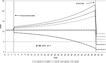
Figure 1a: Rents and Prices
σ=3, α=-.05
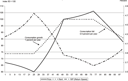
Figure 2: US Demographics with Projections
Population in Thousands
Figure 3: United States: Percent of Population Under Age 5
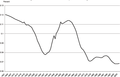
Figure 4: United States: Percent of Population Working Age
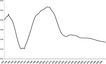
Figure 5: United States: Real House Prices
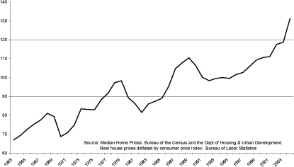
Figure 6: Real Long and Short Interest Rates
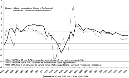
Figure 7: Real House Prices and Model House Prices
No Discounting
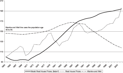
Figure 8: United States: Simulated House Prices
Index 1994 = 100
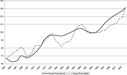
Figure 8a: United States: Simulated House Prices
Index 1994 = 100
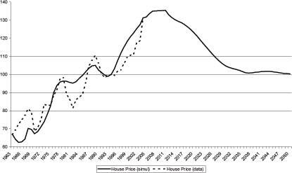
Figure 9: Long-Term Real Interest Rate
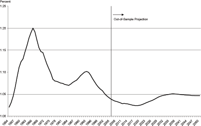
Figure 10: 10 Year Real T-Bill Rate Vs. Model Real Ten Year
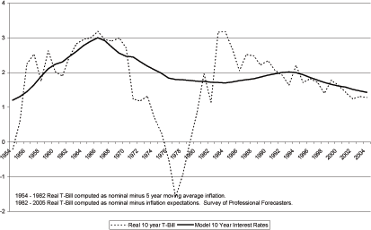
Figure 11: Short-Term Real Interest Rate
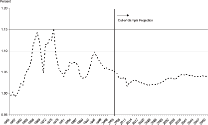
Figure 12: Macroeconomic Volatility
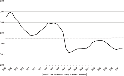
Figure 13: Japan: Simulated and Real House Prices
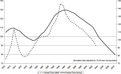
Figure 14: Real House Prices: U.S. vs. U.K.
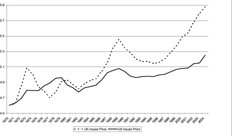
Figure 15: Baby Boom: U.S. vs. U.K.
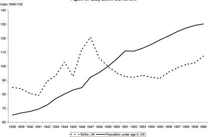
Figure 16: United Kingdom: Simulated and Real House Prices
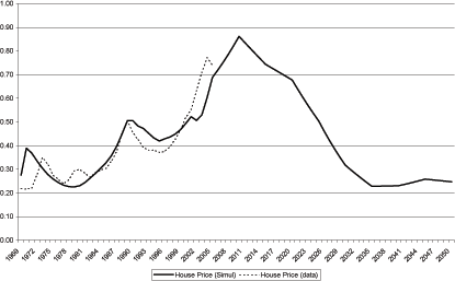
Figure 17: Ireland: Simulated and Real House Prices
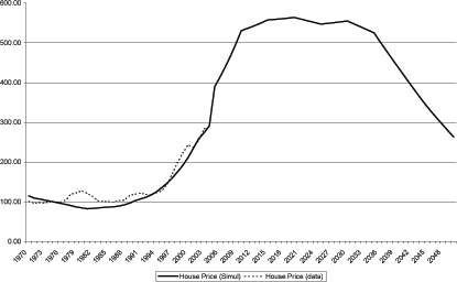
Footnotes
* I would like to thanks Sanjay Chugh, Morris Davis, Linda Kole, Thomas Tallarini, Brian Doyle, Jon Faust, and Sylvain Leduc. Correspondence should be addressed to: Robert F. Martin ([email protected]), Board of Governors of the Federal Reserve System, Washington DC 20551, USA. Return to text
1. The dates for the comparison are chosen to include the dates for which the baby boomers were fully incorporated into the work force. It is worth noting as well that the increase in relative consumption is not calibrated but rather is an implication of holding capital and productivity fixed while adjusting the labor input to replicate the impact of the baby boom. Return to text
2. Any individual agent can transfer output over long periods of time by trading long-lived bonds. Thirty year bonds exist and exhibit fairly liquid markets. However, to undo the effects in the model real output must be physically transferred from today to the future. As the demographic shocks discussed in this paper occur over 30 to 50 year intervals, it is difficult to think of a real asset capable of making this transformation. Think of real capital and assume it depreciates at a mere 5 percent per year. Almost 80 percent of the capital is consumed by depreciation over the 30 year period. On a discounted basis over 95 percent of the capital is eroded. It is in this sense, that the ability to transfer assets to the future is limited. Return to text
3. In actuality, whether or not house prices rise or fall in response to a future fall in output is parameter dependent. I show that this is true if and only if the cross-derivative between consumption of goods and consumption of housing is negative. For CES utility, this implies that the elasticity of intertemporal substitution must be less than the elasticity of intratemporal substitution. It turns out that this is the same requirement for house prices to fall when interest rates rise. Return to text
4. Conditioning on observed productivity shocks would improve the fit of the model. Alternatively, a model with endogenous collateral constraints as in Lustig and Van Nieuwerburgh (20050 would likely improve the ability of the model to replicate the amplitude of he swings in house prices. In this model, the collateral constraints would serve as an accelerator (see Campbell and Hercowitz (2004)). Return to text
5. Of course, researchers have been able to match the individual peaks and by extension match every peak using a unique explanation for each episode (see Ahearne et al. 2005). The common explanations are as follows: 1969 - the expansion associated with the Vietnam war; 1973 - housing as a hedge against inflation; 1979 - change in the U.S. tax code; 1989 - expansion of bank loans; Current - steady low inflation brought about by improved monetary policy. Return to text
6. Long-term real interest rates are defined as 10 year treasury yields adjusted for inflation expectations. For the period 1950 through 1982, I use a backward looking two-year moving average of inflation to proxy for inflation expectations. From 1982 forward, I use the survey of professional forecasters available from the Philadelphia Federal Reserve. Return to text
7. An important exception to this is the study conducted by Mankiw and Weil (1988) which is discussed in the next sub-section. Return to text
8. De Nardi (2001) shows in her dissertation and in subsequent work with Cagetti (2005) that the savings properties of over-lapping generation economies are quite sensitve to the bequest motive. Return to text
9. In a single household, the thought experiment is as follows: A couple with no children has time endowment of 1. A couple with three children (all below working age) was a time endowment of 2/5. A couple with three working children has a time endowment of 5/5. The same household with two retired parents has a time endowment of 3/5. Return to text
10. The pricing kernel is defined in terms of the marginal utility of numeraire consumption. Below in the simulation section, a new pricing kernel is defined, by exploiting the specific functional form, over total consumption. Return to text
11. For ease of exposition, the short cut of considering changes in prices to changes in consumption is used. However, since consumption and output are isomorphic this short cut is without loss of generality. Return to text
12. In the data section below, prices are
typically shown as index values. The degree of freedom offered by
the parameter ![]() makes the indexing without loss
of generality. Return to text
makes the indexing without loss
of generality. Return to text
13. The change in the consumption path is
a zero probability event. The price path shown from date
![]() forward is exactly identical to the price
path which would have occurred had the fall in consumption at date
forward is exactly identical to the price
path which would have occurred had the fall in consumption at date
![]() always been known. The announcement is
treated as an event in this case to highlight the price jump at the
announcement date. Return to
text
always been known. The announcement is
treated as an event in this case to highlight the price jump at the
announcement date. Return to
text
14. Recall, the rental price of housing
in period ![]() is given by
is given by
 Hence, rents are governed by
 ![]() and
and
![]() and the relative size of the two
goods. Notice, the more negative is
and the relative size of the two
goods. Notice, the more negative is ![]() the
more rents fall at date 50 and that rents are absolutely constant
until date 50. Return to text
the
more rents fall at date 50 and that rents are absolutely constant
until date 50. Return to text
15. Note, that the response in interest
rates to a fall in consumption is largely governed by the magnitude
of ![]() As
As ![]() increases, the interest rate become more sensitive to changes in
consumption. Of course, the responsiveness of house prices is also
determined by the responsiveness of interest rates. Return to text
increases, the interest rate become more sensitive to changes in
consumption. Of course, the responsiveness of house prices is also
determined by the responsiveness of interest rates. Return to text
16. Demographic projections are often thought of as highly inaccurate (Porterba (2004)). However, even ex post, the evolution of the age population in the United States appears to be dominated by the baby boom. This dominance remained despite large changes in the pattern of immigration over the post war years. Return to text
17. Greenwood et al. (2002) date the start of the baby boom for the United States in 1936. Indeed, by any measure one might choose - fertility rates, birth rates, population growth - the baby boom is obvious in the data and importantly the baby is not an isolated post-WWII event. Further, as this paper takes the existence of the baby boom as given and merely traces through the impact of the baby boom conditional on its occurring, we also do not dispute Greenwood et al's reason, technological progress, for the boom occurring. Return to text
18. In U.S. data, real rates also rise over this period. This period emphasizes why it is so difficult to use regression analysis to understand the relationship between house prices and interest rates. Regressions over this period, either in actual data or from the model, imply a negative relationship between interest rates and prices. Therefore, inclusion of this period in a study, tends to weaken the implied relationship. This is one of the reasons that Mankiw and Weil did not include interest rates in their study. The interest rate effect would have gone the wrong way. Return to text
19. Goodfriend and King infer the expectations of the Federal Reserve from published minutes and Federal Reserve forecasts. Return to text
20. Japan has experienced a prolonged period of deflation. The GDP deflator for Japan is nearly 14 percent below its 1990 level. Return to text
21. The data, while not exactly comparable, is quite similar in nature to the fertility data presented by Greenwood et. al. (2002) figures 6 and 8. These figures show a protracted hump in fertility rates in the United States and a sharp spike in fertility in the United Kingdom. Return to text
This version is optimized for use by screen readers. Descriptions for all mathematical expressions are provided in LaTex format. A printable pdf version is available. Return to text