Skip to: [Printable Version (PDF)]

Board of Governors of the Federal Reserve System
International Finance Discussion Papers
Number 925, March 2008--- Screen Reader Version*

Bank Integration and Financial Constraints: Evidence from U.S. Firms

Ricardo Correa^*

NOTE: International Finance Discussion Papers are preliminary materials circulated to stimulate discussion and critical comment. References in publications to International Finance Discussion Papers (other than an acknowledgment that the writer has had access to unpublished material) should be cleared with the author or authors. Recent IFDPs are available on the Web at http://www.federalreserve.gov/pubs/ifdp/. This paper can be downloaded without charge from the Social Science Research Network electronic library at http://www.ssrn.com/.

Abstract:

This paper uses data on publicly-traded firms in the U.S. to analyze the effect of interstate bank integration on the financial constraints borrowers face. A firm-level investment equation is estimated in order to test if bank integration reduces the sensitivity of capital expenditures to the level of internal funds. The staggered deregulation of cross-state bank acquisitions that took place in the U.S. between 1978 and 1994 helps estimate the model. Integration decreases financing constraints for bank-dependent firms. The change in firms' access to external finance is explained by an increase in the share of locally headquartered geographically diversified banks.

Keywords: Bank deregulation, investment, financing constraints

JEL classification: G21, G28, G31

This paper presents the first firm-level analysis on the effect of interstate bank integration on firm financial constraints. Between 1976 and 1994, the share of deposits held by Multi-State Banks (MSBs) in the U.S. rose from 12% to 69%. Existing literature suggests that this increase in bank integration through cross-state acquisitions is associated with enhanced bank efficiency (Jayaratne and Strahan (1998)), improved interstate income insurance (Demyanyk, Ostergaard, and Sørensen (2007)), and less state-level business cycle volatility (Morgan, Rime, and Strahan (2004)).¹However, these studies do not consider the impact of bank integration on individual firms. This paper fills that void by asking two questions: did bank integration reduce financing constraints for publicly-traded firms? Was this effect the result of bank geographical diversification or the introduction of more efficient banking practices in local markets?

Bank integration has an ambiguous effect on firms' access to credit. On the one hand, interstate bank entry through acquisitions improves local competition in the retail loan market (Park and Pennacchi (2008)), reduces inefficiencies associated with entrenched managers (Hubbard and Palia (1995)), and increases the frequency of new local bank charters (Berger et al. (2004)). Moreover, geographical diversification allows banks to engage in riskier lending without increasing their overall risk (Demsetz and Strahan (1997)). On the other hand, MSB entry may reduce the flow of credit to more obscure, bank-dependent firms. Large-size banks rely on "hard information" to assess the credit-worthiness of their borrowers. As small and intermediate banks are acquired by out-of-state MSBs, bank financing decreases for bank-dependent firms (Keeton (1996)). This conflicting evidence suggests that the relation between bank integration and firm financing constraints has to be determined empirically.

The U.S. is a good place to study the effect of bank integration for three reasons. First, bank regulation before the 1970s created 50 isolated banking systems with idiosyncratic characteristics. These differences were translated into varying levels of firms' access to credit before deregulation. Second, when states changed their regulatory restrictions they did so at different points in time. Because the U.S. experienced other regulatory changes that affected all states simultaneously, the staggered process of interstate entry deregulation permits identification.² Finally, although U.S. states have their own laws and differ in their economic structure, these differences are minor compared to differences between countries. Hence it is simpler to control for state specific effects.

There is no comprehensive data source containing information on bank borrowing at the firm level for the period in which interstate entry deregulation was implemented in the U.S.³ Therefore, I use an indirect method to asses the effect of bank integration on firms' access to bank credit. The methodology follows the well established literature on investment with financing constraints.⁴ An Euler equation for investment is estimated using firm-level data on publicly-traded firms in the U.S. manufacturing sector for the period between 1976 and 1994. Since the decision to deregulate cross-state bank entry is exogenous to the firm, this paper takes advantage of the staggered banking liberalization that took place across states to estimate the impact of state laws on borrower financing constraints.

First, I investigate whether bank integration had an effect on external financing for the complete sample of publicly-traded firms with information before and after interstate bank entry deregulation. As expected, bank integration had a small effect on the sensitivity of investment to internal funds for this sample of firms. Large corporations are able to access public debt markets or issue equity instead of using bank debt (Bolton and Freixas (2000)). Banking deregulation does not change the financing conditions that these firms face. In contrast, firms with more informational asymmetries are more likely to use bank credit to finance their investment expenditures. A change in the banking sector should have a significant effect on this group of bank-dependent firms.

The next step is to test whether bank-dependent firms benefit from bank integration. I define bank dependence in terms of the firms' size or access to the public debt market. The estimations confirm that bank integration, measured by an indicator variable denoting interstate bank entry deregulation, has a significant effect on bank-dependent publicly-traded firms. The sensitivity of investment to internal funds is significantly weaker after interstate agreements permitting cross-state acquisitions are passed. Using the market share of MSBs in local markets as the bank integration measure yields similar results.

After determining that bank integration decreases firm financing constraints, I analyze the factors that account for the reduction in these financing frictions. Financial constraints are explained by informational asymmetries between borrowers and lenders. Banks use monitoring and screening mechanisms to reduce these informational problems. But if banks are financially constrained themselves, their impact on the reduction of firms' financing frictions might be limited. Through cross-state acquisitions, local banks are able to diversify geographical risks (Strahan (2006)), and establish internal capital markets to finance loan growth (Houston and James (1998), Houston, James, and Marcus (1997)). Therefore, bank integration allows local MSBs to provide better financing terms to firms with whom they have an established lending relationship. I find that an increase in the market share of locally headquartered MSBs has a stronger effect on firms' access to credit than the entry of out-of-state MSBs. This evidence allows me to conjecture that changes at local financial institutions are more important in reducing financing constraints than the introduction of new lending practices by out-of-state banks.

In the last set of estimations, I use data on firms' short-term borrowing spreads to test if bank integration has a direct effect on firms' financing costs. According to the investment model, a decrease in firm financing constraints has to be accompanied by an increase in firms' access to external funds. As borrowing costs decrease, bank-dependent firms are able to use bank credit to finance their investment expenditures. I find that spreads decrease significantly for bank-dependent firms after interstate entry deregulation. In particular, a 30 percentage point increase in the MSBs' market share reduces bank-dependent firms' short-term borrowing spreads by 30%.

The literature on bank integration and firms' access to credit has focused on the relationship between banking consolidation and banks' supply of credit (Berger, Demsetz, and Strahan (1999)). Berger et al. (1998) study the dynamic effect of banking consolidation on small business lending, while Erel (2007) analyzes the change in loan spreads charged to firms after a bank merger or acquisition. In a closely related paper, Houston and James (2001) find that firm financing constraints vary systematically with the reliance on bank debt and the number of banking relationships held by firms. I build on this evidence and establish that bank integration through cross-state consolidation-altering banking relationships in the process-has a significant effect on bank-dependent firms' access to credit.

Lastly, this paper contributes to the literature on investment with financing constraints by exploiting the interstate entry deregulation episode that took place in the U.S. in the 1980s. Rauh (2006) uses exogenous shocks to the firms' internal funds to identify if firms are dependent on this source of financing. In contrast, I take advantage of an exogenous shock to the primary source of external finance, to test whether this change has an effect on the use of internal resources to finance investment. In addition, I provide an explanation for the downward trend in the sensitivity of investment to internal funds documented in Allayannis and Mozumdar (2004).

The rest of the paper is organized as follows. Section I provides an overview of the history of banking deregulation in the U.S., and outlines the links between bank integration and firms' access to credit. Section II describes the empirical strategy and the data used in the estimations. Section III presents the main results. Section IV uses a difference-in-difference analysis to study the effects of bank integration on firms' short-term borrowing costs. Finally, section V concludes.

1  Background

1.1  Recent History of Banking Deregulation in the U.S.

Starting with the McFadden Act of 1927, the U.S. endured a period of restrictions on branching and interstate acquisitions that lasted until the last decades of the twentieth century. The first restrictions lifted were those that limited intrastate branching. By 1974, 13 states had already allowed unrestricted branching within their borders. In the next two decades, 35 more states eliminated partially or all restrictions on intrastate branching. Differences in states' willingness to allow branch networks sustained the development of very diverse bank systems across states, where some of them allowed only unit banking while other states permitted statewide branching.

The Douglas Amendment to the Bank Holding Company act of 1956 prohibited Bank Holding Companies (BHCs) from establishing or purchasing bank subsidiaries across state lines unless the state of the target bank authorized the transaction. These restrictions remained until Maine passed a law allowing out-of-state BHCs to purchase local banks if the "home" state of the BHC reciprocated. No state followed Maine's lead in opening their financial sector to out-of-state banks until 1982 when Alaska and New York passed similar laws. The same year, as part of the Garn-St Germain Act, federal legislators amended the Bank Holding Company Act to allow failed banks to be acquired by any BHC, regardless of origin and state laws. This regulatory change, coupled with a series of bank and thrift failures during the 1980s, triggered a wave of interstate agreements that effectively permitted banking at the national level.

Before 1994, 49 states and the District of Columbia had deregulated their banking markets allowing out-of-state entry. Typically, acquisitions by out-of-state BHCs were limited to banks from same-region states although some states were open to nationwide entry. Interstate branching was permitted nationwide with the Riegle-Neal Interstate Banking and Branching Efficiency Act, which became effective in June 1997. Some states took advantage of a clause in the Act and opted out at an earlier date.⁵

1.2  What is the Link Between Bank Integration and Firms' Access to Credit?

Interstate bank entry deregulation in the U.S. had significant effects on the real economy.
At the state level, Strahan (2003) finds that interstate entry deregulation increased incorporations by state and reduced the comovement between state growth and local bank performance. In a study on income insurance, Demyanyk, Ostergaard, and Sørensen (2007) show that deregulation, measured as the combination of intra- and interstate deregulation, decreased the correlation between personal income and state-specific shocks to output. Their result is stronger for proprietor income than wage income. The authors explain this effect by the closer relationship between banks and small businesses. This outcome is connected to Morgan, Rime, and Strahan's (2004) finding that geographical bank integration reduced employment volatility within states. A decline in the impact of bank capital shocks on state activity explains this increased stability in the economic environment. At the micro level, Correa and Suarez (2008) document a decrease in publicly-traded firms' real and financial volatility after cross-state bank entry deregulation was enacted. In the rest of the section, I outline the direct links between bank integration and firms' access to credit.

The first effect of bank entry deregulation on firms' access to credit is channeled through its impact on bank efficiency. Jayaratne and Strahan (1998) find substantial reductions in loan losses and operating costs after cross-state acquisitions were permitted. Hubbard and Palia (1995) show that turnover and the sensitivity of pay to performance for bank senior executives increased after states allowed interstate banking. This change is interpreted as a tightening in management discipline due to an increased risk of takeovers. Lastly, Stiroh and Strahan (2003) find a stronger link between performance and market share after deregulation. This is attributed to the competitive reallocation of assets to better performers. The empirical evidence points to an increase in bank efficiency after cross-state deregulation. The question that emerges is if this increase in bank efficiency had an effect on firms by granting them greater access to credit.

Bank efficiency is not the only factor changed by interstate bank entry deregulation. Bank integration also allows banks to diversify their loan portfolio geographically. Demsetz and Strahan (1997) find that large diversified BHCs are able to increase business loans while operating with higher leverage. In a set of related papers, Houston, James, and Marcus (1997) and Houston and James (1998) argue that BHCs use internal capital markets to allocate resources amongst their subsidiaries. These internal markets are shown to isolate the effect of local economic conditions on affiliated banks' lending activity (Ashcraft (2006)). The net benefit for firms is an increase in the availability of banks' loanable funds and a decrease in the sensitivity of credit supply to local economic activity.

The literature has also addressed the negative consequences of bank integration. The main concern is that bank consolidation through acquisitions may terminate established banking relationships between borrowers and lenders. Berger and Udell (1996) show that an increase in average bank size in a specific market due to consolidation has the effect of decreasing bank lending to small businesses. Peek and Rosengren (1998) expand on this idea and find that acquired banks adopt the lending patterns of the acquirer after a merger.⁶ If the acquiring bank has a bias for large-firm lending, the target will adopt the same strategy. The international evidence shows a similar pattern of negative outcomes after banking consolidation. Karceski, Ongena, and Smith (2005) use a sample of Norwegian publicly-traded firms to study the effect of bank mergers and acquisitions (M&As) on their borrowers' stock prices. The authors find that small borrowers are the most affected after mergers and are also the least likely to switch to other banks for their credit requirements. In a detailed study of Italian firms, Bonaccorsi Di Patti and Gobbi (2007) show a decrease in the amount that firms borrow from banks involved in a merger as a bidder or a target.⁷ This effect dissipates after 3 years, possibly explained by firms switching their business to other banks, as it has been the case in the U.S. (Berger et al. (1998)).

The conflicting evidence discussed in this section makes the question on the effect of bank integration on firms' access to credit an empirical task. The deregulation of cross-state bank acquisitions in the U.S. provides a useful setting to study this link. In addition, I test if changes in firm financing due to bank integration are explained by local banks diversifying their assets geographically, or if out-of-state bank entry determines the change in firms' access to external finance.

2  Testing Framework and Data

2.1  Estimation Methodology

Information on the demand of bank loans by firms starting in the pre-deregulation period is scarce and incomplete. This factor limits the options available to estimate the impact of interstate bank entry deregulation on firms' access to credit. In this study, I use an indirect method to assess the effect of changes in bank integration on firm financing. I estimate a reduced form equation from a model of investment with financial frictions. The model assumes that shareholders (managers) maximize the present value of the firm, which is the expected discounted value of dividends, subject to capital accumulation and external financing constraints.⁸ After making some simplifying assumptions and linearizing the euler equation implied by the model, I arrive at the following estimating equation:$^{ }$⁹

$$\begin{array}[c]{c} \frac{I_{it} }{K_{it-1} }=\alpha_{0} +\alpha_{1} \frac{I_{it-1} }{K_{it-2} }+\alpha_{2} \frac{Sales_{it-1} }{K_{it-1} }+\alpha_{3} \frac{Cash_{it-1} }{K_{it-1} }+\alpha_{4} \frac{Cash_{it-1} }{K_{it-1} }\times Intg_{jt}\\ +\alpha_{5} Intg_{jt} +\beta Z_{jt} +f_{i} +h_{t} +\varepsilon_{it}\\ \end{array}$$ (1)

where $I_{it}$ represents investment for firm $i$ at time $t$; $K_{it-1}$ is the stock of capital at the beginning of period $t$; Sales $_{it-1}/K_{it-1}$ is a proxy for the marginal profit of capital; Cash $_{it-1}/K_{it-1}$ measures the level of internal funds held by the firm at the beginning of time $t$; bank integration in state $j$ at time $t$ is given by Intg$_{jt}$; $f_{i}$ and $h_{t}$ are fixed and time effects, respectively; $Z_{jt}$ is a vector of state-level variables capturing aggregate shocks by state. The error term $\varepsilon$$_{it}$ is orthogonal to any information available at the time when the investment decision is made.

In an environment with perfect capital markets, a firm's investment decision depends on the marginal profitability of capital, represented in (1) by Sales $_{it-1}/K_{it-1}$. But a series of empirical studies have shown that investment expenditures are also correlated to the level of internal funds held by the firm (Gilchrist and Himmelberg (1998) and Love (2003)). This is explained in the underlying model-from which (1) is derived-by a shadow price differential between external and internal finance. Firms with limited access to external sources of funding have to accumulate liquid assets to finance their investments.¹⁰ The degree of reliance on internal funds varies with the firms' information asymmetries.

This setting provides a role for banks, as their existence is based on the capacity to minimize information problems through the use of monitoring and screening mechanisms (Diamond (1991)). Bank entry deregulation has an effect on financing constraints by changing the cost of external sources of finance for firms with higher degrees of informational asymmetries. As competition, diversification, and technological improvements are enhanced in previously isolated banking markets, the availability of external funds should increase for this type of bank-dependent firms. However, as out-of-state banks enter local markets through acquisitions, some of the information available in established banking relationships might be lost, and this could increase the cost of financing. Then, the question of the effect of bank integration on financial constraints becomes empirical, and is tested using the coefficients estimated from (1). The test is formally stated as:

$$H_{0} :\alpha_{3} \ge0\; \;\alpha_{4} <0$$ (2)

This hypothesis implies that some firms become less dependent on internal funds to finance their expenditures after bank entry deregulation, or that financial constraints decrease as bank integration increases.

Some empirical and theoretical studies have criticized the methodology used in this paper.¹¹Their main concern is that the sensitivity of investment to internal funds-commonly proxied by cash flow-could be explained by factors not related to firm financing constraints. Houston and James (2001) deal with this issue by analyzing the characteristics of bank-dependent firms, and comparing them to those of firms with access to multiple sources of credit. These authors find that bank-dependent firms, especially with single banking relationships, hold higher proportions of cash relative to capital, and have lower leverage ratios and dividend payouts. This evidence suggests that bank-dependent firms face greater financing constraints relative to firms with access to wider funding sources.

I deal with the issues regarding this empirical approach by testing the null hypothesis in (2) for a group of bank-dependent firms. Then I contrast these results with those of firms that do not rely on banks as their source of external finance. Furthermore, the use of an exogenous event like the deregulation of out-of-state bank entry, isolates the effect of changes in the costs of external funds on the sensitivity of investment to cash. The resulting difference-in-difference analysis disentangles the change in the investment-cash sensitivity that is explained by bank-dependent firms' access to external finance from other factors. This method addresses some of the identification problems outlined in the literature on investment with financing constraints.

2.2  Econometric Issues

There are two issues that need to be addressed to estimate the empirical model in equation (1). First, fixed effects ($f_{i})$ are correlated with regressors due to the presence of lags of the dependent variable in the estimating equation. This specification requires panel data techniques to obtain consistent estimates of the coefficients. Second, some of the explanatory variables in (1) could be simultaneously determined with the dependent variable. A General Method of Moments (GMM) procedure implemented as instrumental variables is used to control for this problem.

In order to solve the first issue, unobservable fixed effects are eliminated by transforming all variables using a first differencing procedure.¹² This technique induces endogeneity between the difference of the lagged dependent variable and the idiosyncratic component of the error term; the same applies to predetermined variables like Sales $_{it-1}/K_{ it-1}$, Cash $_{ it-1}/K_{ it-1}$, and this variable's interaction with the bank integration proxy. This problem leads to the second solution: I estimate (1) using system GMM with an optimal weighting matrix.¹³

As it was discussed in the previous section, $\varepsilon$$_{it}$ is orthogonal to any information available when the investment decision is made. Firms are assumed to determine the amount they are going to invest in year $t$ at the beginning of the period. Taking into account that firms report their information at the end of the year, all information available to managers will be dated $t-1$. As a result, the orthogonality conditions are given by $E(X^{\prime}_{it}$ $\varepsilon$$_{is})=0$ for all $s$>$t+1$, where $X$ is the vector of instruments.¹⁴ The estimator is implemented using $t-3$ and $t-4$ lags of the untransformed variables as instruments in the difference equation, and the same lags of differenced variables in the levels equation. I include all variables as instruments in the regressions, plus industry dummies at the 2 digit SIC level.

I conduct two tests to assess the validity of the instruments used in the empirical estimations. The first test, developed by Arellano and Bond (1991), evaluates if there is no first-order autocorrelation in the idiosyncratic disturbances ( $\varepsilon$$_{it})$. This test determines if lags one and deeper of the explanatory variables are valid instruments, as they are not endogenous to lagged values of $\varepsilon$$_{it}$. I report the tests of first- and second-order autocorrelation on first-differences of the idiosyncratic disturbances. The statistic on second-order autocorrelation is the most relevant, as it is equivalent to a test of first-order autocorrelation for levels of $\varepsilon$$_{it}$. The second test, called the J-statistic, was proposed by Hansen (1982) and evaluates the joint validity of the moment conditions. Under the null hypothesis, it is distributed as $\chi^{2}$ with degrees of freedom equal to the number of overidentifying restrictions.

Lastly, I report second stage coefficients and standard errors using Windmeijer's (2005) small-sample correction method.

2.3  Bank Data

Bank integration during the 1970s and 1980s is measured using four different proxies. The first measure is an indicator variable equaling one when a state passed an interstate banking agreement with other states, and zero otherwise. Table I reports the dates when these agreements were enacted in each state.¹⁵ Maine passed the first interstate agreement in 1978 followed by Alaska and New York in 1982. On aggregate, 18 agreements were approved before 1985, 26 between 1986 and 1990, and 4 more before the Riegle-Neal Interstate Banking and Branching Act passed in 1994.¹⁶

In addition to the indicator variable, there are three measures computed using commercial banks' balance sheet items. These integration measures are the share of deposits, commercial and industrial loans (C&I), and assets controlled by MSBs in each state. An MSB is defined as a bank with holdings in more than one state. For the period between 1976 and 1994, financial data is taken from the quarterly Reports of Condition and Income (Call Reports) compiled by the Federal Deposit Insurance Corporation (FDIC), the Office of the Comptroller of the Currency (OCC), and the Federal Reserve System.

Figure 1 shows the evolution of the three continuous integration measures in the last three decades. Bank integration, as measured by these shares, remained stable and close to 10% before 1982. From this year onwards, there was a considerable increase in the share of assets, C&I loans, and deposits held by MSBs, reaching the 60% mark in 1994. This pattern is consistent with the passage of interstate agreements beginning in 1982.

Table I shows the average share of deposits in MSBs by state before and after 1982. Most states have very small MSB penetration prior to this year. Some exceptions are found in western and midwestern states, explained by grandfathered agreements prior to the passage of the Bank Holding Company Act of 1956, which explicitly prohibited interstate banking. The mean of the share of deposits held in MSBs increased from 9% before 1982 to 41% after out-of-state bank entry was deregulated in 1982.

In the last column of Table I, I report the average post-deregulation difference between the share of deposits-relative to total deposits in each state-held in local MSBs and the share held in out-of-state MSBs. This measure shows to what extent a state's banking sector is dominated by local "exporters" of banking services, as opposed to their out-of-state counterparts. For example, states like North Carolina and Michigan have banking sectors that are mostly serviced by MSBs that have their headquarters in the state. In contrast, a large share of deposits in Nevada and Washington are held in banks owned by out-of-state MSBs.

Finally, as a robustness check I include a variable to control for bank concentration in some of the estimations. The Herfindahl-Hirschman Index for deposits is computed at the state level between 1976 and 1994.¹⁷ Then, I define an indicator variable by state and year, equaling one when the Herfindahl-Hirschman Index is above the median (914). Although not a perfect measure, it captures the banking sector's market structure.

2.4  Firm Data

Firm level data is compiled from the Compustat database, which contains Balance Sheet and Income Statements for publicly-traded firms.¹⁸ The sample consists of U.S. manufacturing firms (SIC codes 2000 to 3999) between 1976 and 1994. The main advantage of using Compustat is that it covers firms before and after interstate banking deregulation took place. This information allows me to measure the change in financial constraints due to bank integration.

A firm's "home" state is determined by the location of its corporate headquarters or home office. Compustat's geographic information reports the location of firms headquarters only for the latest year available in the database. To determine whether a firm was affected by bank entry deregulation, I have to find the actual historical location of its headquarters. For this purpose, I use data from Compact Disclosure between 1988 and 1994. This source contains extracts from SEC filings updated every month, including the firm's address. With this information I establish the state where a firm was headquartered during the deregulation period.¹⁹

After the geographical location, firms' dependence on bank financing is the other relevant characteristic used in the empirical tests. Compustat does not itemize the amount of bank debt held by firms. I resort to two proxies to determine a firm's level of bank dependence: one is based on firms' size and the other, on the use of public corporate debt. Small firms and firms with no access to public debt markets are usually defined in the literature as being a priori financially constrained (Almeida, Campello, and Weisbach (2004)). Moreover, Houston and James (1996) find that firms without public debt are smaller and hold more bank debt. Dividing the sample using size and public debt access, allows me to focus on those firms that are more likely to rely on internal funds for investment-financing, and at the same time, be affected by bank entry deregulation.

I define the first bank dependence indicator by using the firms' history of credit ratings and issues between 1970 and 1994. A firm is classified as being bank-dependent if it did not issue debt nor had any credit ratings in this period, and held an average positive total debt balance. Bond and commercial paper credit rating information is retrieved from Compustat. Bond and commercial paper issues are obtained from the Mergent Fixed Income Security Database (FISD) and Moody's Default Risk Service (DRS) Database. About two-thirds of firms in the sample are classified as being bank-dependent.²⁰

For the second classification criterion, firm size, I use the beginning-of-period assets in 1995 U.S. dollars.²¹ Firms are allocated into groups according to the median value of assets in the state where their headquarters are located, and into terciles using the full sample of firms. The number of firms classified as bank-dependent varies by year.

All firm-year observations with complete data on the required variables are used in the sample. A minimum coverage of four years of data is set for each firm due to the loss of observations implicit in the estimation procedure. Furthermore, a firm is required to have at least 2 years of data before and after an interstate agreement is signed by its "home" state.²² However, it is necessary to delete more firms due to possible outliers in the sample explained by acquisitions, revaluation of assets, or problems with the data. The result of this process is an unbalanced panel of firms for the period between 1976 and 1994. Details on sample selection and outlier rules are given in Appendix 2.

Table II reports the number of firms and observations by state used in the main estimations. A total of 1,715 firms and 25,667 firm-year observations are included in the sample with average data coverage of 15 years per firm. Companies are unevenly distributed across states, with California and New York accounting for 26% of the sample.

I calculate the necessary variables to estimate equation (1) from this firm-level dataset. As discussed in section II.B, investment is assumed to be determined at the beginning of period $t$. Since accounting data are stated at the end of each period $t$, end-of-period $t-1$ data on sales, cash stock, and capital are used as regressors.²³ Other variables are defined in Appendix 3.

Panel A in Table III shows descriptive statistics for the main variables and all firms included in the sample. The median firm has real assets of 112 million (1995 US dollars). Panels B and C include the same statistics for the sub-samples of firms without and with access to public debt. The group of firms with no access to public debt, or bank-dependent, has median assets of 44 million, considerably lower and statistically different to the 793 million in assets of firms with access to public debt. Additionally, cash holdings are larger and leverage lower for bank-dependent firms.²⁴ These findings indicate that bank-dependent firms hold more liquidity and acquire less debt, which suggest that this group of firms face greater external financing constraints (Houston and James (2001)).

The last column in panels A through C shows the spread between the average short term interest rate paid by firms and the prime rate.²⁵ Bank-dependent firms have a median spread that is 40 basis points higher than firms with access to public debt markets. This difference is statistically significant, and reinforces the claim that bank-dependent firms are financially constrained. They have to pay higher rates to receive bank credit. The estimations in the following sections test if banking deregulation decreased the rates paid for external financing and reduced financing constraints.

3  Results

3.1  Main Results

Tables IV through VI show the main results of the paper based on the model in equation (1). The first column in Table IV uses the bank integration measure defined as an indicator variable equal to one after a state passes an interstate agreement law. The coefficients on sales and lagged investment have the predicted sign and are significant at the 1% level. The coefficients I want to test are cash stock and its interaction with the bank integration variable. The sign of these two coefficients are in line with the hypothesis stated in (2), and are significant at the 5% and 10% level. This result implies that after interstate bank entry is permitted, the cash-investment sensitivity decreases for this sample of publicly-traded firms.

In columns (2), (3), and (4), bank integration is measured by using continuous variables representing the share of deposits, C&I loans, and assets held by MSBs. The effect of bank integration, proxied by these variables, on the cash-investment sensitivity is weaker. Although the coefficients on the measure of internal funds and its interaction with bank integration have the predicted signs, the net effect after adding both terms is positive and significantly different from zero.

It is not surprising to observe a weak change in the sensitivity of investment to internal funds, as bank integration increases, using the full sample of firms. Bank integration is expected to have different effects depending on the size and the sources of funding available to each firm-amongst other characteristics. Large publicly-traded firms are able to access public debt markets, limiting their reliance on bank debt to finance investments (Houston and James (1996)). Any change in bank regulation has a marginal effect on this set of businesses. In contrast, bank-dependent firms use bank debt more frequently to mitigate information asymmetries that arise in the relation between lenders and borrowers.²⁶ The reliance on bank debt will likely strengthen the effect of bank deregulation on this particular sub-sample of publicly-traded borrowers.

In Table V, I estimate the model used in columns (1) and (2) of Table IV, but I divide the sample by the firms' access to public debt markets. A firm is classified as bank-dependent, if it had average positive debt, and did not issue nor had ratings of commercial paper or bonds between 1970 and 1994. Results in columns (1) and (3), show that the cash-investment sensitivity is positive and significant for bank-dependent firms. This result is consistent with previous evidence on firm financial constraints (Houston and James (2001)), as this group of bank-dependent firms is more likely to face greater information asymmetries when accessing external sources of finance.

The most relevant result in these estimations is the negative and significant value for the coefficients on the interaction between cash stock and the measures of bank integration. The sum of the coefficient for cash stock and the coefficient on its interaction with bank integration is not statistically different from zero for bank-dependent firms. This result is robust to the use of the deregulation indicator variable and the share of deposits held by MSBs as the bank integration proxy.²⁷ Financial constraints decrease significantly for bank-dependent firms in the post-deregulation period, as the sensitivity of investment to internal funds becomes negligible.

Results are different for firms with access to public debt markets. The sensitivity of investment to internal funds is not significantly different from zero, and it does not change with bank integration, as shown by the coefficients in columns (2) and (4). The results for this sample of firms have to be treated with caution. The reported Hansen test statistic for over-identification is used to verify the validity of the model. In the two specifications, the p-value reported indicates that the null hypothesis that the over-identifying restrictions are valid can be rejected. This evidence suggests that the model of investment with financing constraints does not apply to firms with diversified sources of financing.

Table VI reports results for firms divided by size. Firms are defined as bank-dependent if their assets (in 1995 U.S. dollars) are below the sample median in the state where they are headquartered, or if their assets are in the bottom tercile of the distribution for the full sample of firms. Results from this set of estimations show that integration reduces financing constraints for small publicly-traded firms. This is corroborated by the negative and significant coefficient on the interaction of bank integration and cash for the estimations including bank-dependent firms. In contrast, large publicly-traded firms do not exhibit a significant change in their cash-investment sensitivities due to banking deregulation. As it was the case for firms with access to public debt markets, estimations including large firms are not well specified as signaled by the Hansen test.

The results in this section do not reject the null hypothesis stated in (2) for bank-dependent firms. Bank integration reduces financing constraints for firms with significant informational asymmetries. These findings are consistent with the decline in the sensitivity of investment to internal funds documented in Allayannis and Mozumdar (2004) for the last half of the 1980s and the beginning of the 1990s. As it is shown above, this trend is explained by bank entry deregulation and the subsequent integration of the banking sector.

3.2  What Explains the Reduction in Firms Financing Constraints?

This section explores the mechanisms through which bank integration reduces firm financing constraints. In particular, I test if bank-dependent firms benefit from the increased presence of local MSBs, as opposed to the entry of out-of-state MSBs. I split the bank integration measure in two components depending on the MSBs' geographical location to assess the effect of local versus out-of-state banks on firm financing constraints. The first indicator is the share of deposits (C&I loans)-out of the total value of deposits (C&I loans) in the state-held by local banks with subsidiaries in other states. This measure is called the Share of Banking Exporters. Similarly, I use the share of deposits (C&I loans) held in the host-state by financial institutions owned by BHCs with headquarters located outside the state to determine the effect of out-of-state bank penetration on firm financing constraints. This indicator is labeled the Share of Banking Importers. The bank integration variable (Intg) in (1) is proxied by these two measures. A test on the significance of their coefficients provides additional information on the change in the cash-investment sensitivity caused by bank entry deregulation.

Out-of-state bank entry has an effect on the availability of firm financing through two channels. First, there is a direct effect if larger and more advanced out-of-state institutions introduce better monitoring and screening technologies increasing the set of firms able to acquire bank credit.²⁸ The downside of an increase in out-of-state MSB presence in local markets is the possible loss of established banking relationship. As out-of-state banks enter local markets through cross-state deals, the acquired banks start using "hard" information to assess the creditworthiness of the firms. More opaque bank-dependent firms might lose access to banks that are targets in cross-state deals after deregulation. I determine the net impact of these contrasting effects by testing the significance and sign of the coefficient on the interaction between cash and the Share of Banking Importers.

Bank integration has a second effect on local firm financing that works through an indirect channel. Interstate bank entry deregulation allows MSBs to diversify their assets geographically across states, minimizing the impact of state-level idiosyncratic credit risks. Geographically diversified banks are able to increase the amount of business loans in their portfolio and reduce the premium on external finance faced by local firms.²⁹ In addition, it has been shown that banks that are affiliated to a BHC have access to internal resources available to all subsidiaries belonging to the same financial institution. An internal capital market enables banks to allocate capital within the organization and lend funds to firms with positive net present value projects in any state.³⁰ Although, out-of-state MSBs benefit from geographical diversification and internal credit markets, most of the impact is likely to be observed in the lending behavior of local MSBs. Banks with established lending relationships, but constrained before bank entry deregulation, increase local lending as they diversify risks and allocate resources according to the needs across subsidiaries. Bank integration is expected to reduce the external financing frictions faced by firms in the home-state of the diversified bank. The net effect of geographical diversification and internal markets is tested using the coefficient on the interaction between cash and the Share of Banking Exporters.

Table VII shows the results of estimating the investment equation in (1) for bank-dependent firms. The bank integration measure takes into account the geographical location of banks' headquarters. The hypotheses outlined above are tested using the coefficients on the interaction between cash stock and the two bank integration measures. The sensitivity of investment to cash decreases significantly with an increase in the share of deposits (C&I loans) held by local MSBs. This result is consistent across the different bank dependence definitions. In contrast, the entry of out-of-state MSBs has limited effect on firm financing constraints. The interaction between cash and the Share of Banking Importers is negative in most of the estimations but not significant.

These results suggest that the observed effect of interstate bank entry deregulation on financing constraints-documented in the previous section-is explained by the MSBs local lending. As these institutions expand nationally, they are able to diversify risks associated with their geographical location. Conversely, out-of-state bank presence does not have a significant effect on firms' external financing patterns. As it was explained above, diversification and new technological improvements increase the potential amount that MSBs are able to lend. But cross-state bank acquisitions might destroy established banking relationships reducing the positive impact of interstate bank entry. This is particularly relevant for bank-dependent firms with limited access to other sources of financing.

3.3  Sensitivity Analysis

Tables VIII and IX display the results of sensitivity tests that assess the robustness of the key estimations reported in the previous sections. Variants of the model outlined in (1) are estimated including additional controls, modifying the definition of the variables included, and changing the sample used in the estimations. Robustness checks are shown for the sample of bank-dependent firms without access to public debt markets. Unreported results are similar for bank-dependent firms classified by size.

In the first two columns of Table VIII, I control for bank concentration at the state level. Bank concentration is defined as an indicator variable equaling one if the Herfindahl-Hirschman Index for deposits in a state is above the median in a year. The inclusion of this variable addresses the potential changes in market structure due to bank integration.³¹ The effect of bank concentration on financing constraints is likely to be minor, as interstate bank entry takes place when an out-of-state bank acquires an existing local institution. The target and acquirer are located in different markets; thus, the change in bank concentration at the state level in the short-run is minimal. The results shown in the table confirm the previous findings that bank integration, and not changes in market structure, has a significant effect on the cash-investment sensitivity.

I add leverage to the main equation in (1), defined as total debt by the book value of assets, and show the results in columns (3) and (4). The coefficient on leverage is negative and significant, but the sensitivity of investment to cash is still shown to decrease with bank integration. In columns (5) and (6) Sales/K is replaced by a measure of Tobin's Q as proxy for the marginal profitability of capital. Tobin's Q is defined as the ratio of market value plus book value of assets minus common equity and deferred taxes by the book value of assets. The coefficient on Tobin's Q is positive and significant, and the results on the bank integration measures remain unchanged.

In Table IX I use different sample selection criteria to control for potential biases. The first issue is the possible confounding effects of both intrastate and interstate entry deregulation in the banking sector. Jayaratne and Strahan (1996, 1998) show that intrastate deregulation had a significant effect on income growth and bank efficiency at the state level. Following a pattern similar to that of interstate deregulation, states lifted branching restrictions within the state at different points in time. In columns (4) and (5) I exclude firms located in states where intra- and interstate reforms were implemented within one year.³² Results show that interstate deregulation significantly reduced firm financial constraints in this smaller sample.

The estimations in columns (3) and (4) address the disparity in the number of firms across states observed in Table II. California and New York account for about one-fourth of the firms and observations in the sample. These states will overweight in the cross-state regressions and could prevent smaller states from influencing the coefficients. I exclude firms in California and New York from the estimating sample to check if this sampling effect has an impact on the main results. The coefficients of interest, the interactions between cash stock and the bank integration measures, are negative, significant, and of the same magnitude as the ones observed in the main estimations.³³ Finally, I relax the restriction on including firms with non-missing observations before and after interstate entry deregulation in their home state. The new sample includes firms with at least 4 consecutive years of non-missing observations. As it is shown in columns (5) and (6), the coefficients on the interaction between cash and bank integration are negative and significant. The value of these coefficients is smaller relative to the magnitudes observed using the constrained sample.

I also perform a series of unreported robustness checks. Equation (1) is estimated using different specifications. Instead of first-differencing all variables, I use a forward-mean differencing procedure to remove fixed effects. In other tests, I estimate the model without the equation in levels and using different numbers of lags included as instruments. Finally, I replace the time-varying state-level controls for state-time fixed effects. These additional sensitivity tests confirm the findings on the bank integration effect.

4  Bank Integration and Firms' Short-Term Borrowing Costs

The results from the investment model documented in the previous section show a significant decrease in firm financing constraints explained by an increase in bank integration. In this section, I test if the reduction in the reliance on internal funds to finance investment expenditures is explained by a decrease in the cost of external finance as the theory predicts. There is no comprehensive source of information containing firms' external financing costs going back to the 1980s. I use the average interest rate on short-term borrowing as a proxy for the firms' costs of bank financing. This variable is collected by Compustat from annual 10-K SEC filings, and mainly reflects the firms' cost of outstanding lines of credit.³⁴

The theoretical literature on lines of credit argues that this form of financing solves some of the external finance frictions faced by firms. A committed line of credit ensures that funds are going to be available when firms have the opportunity to invest in valuable projects (Martin and Santomero (1997)). Sufi (2007) finds a close relationship between access to lines of credit and firm financing constraints. Corporations with this type of credit commitment from banks are able to hold less cash out of their cash flow for investment expenditures and liquidity management. A reduction in the cost and increase in access to lines of credit due to bank integration should have a significant effect on the sensitivity of investment to internal funds.

Table X shows the results of a difference-in-difference analysis on the cost of bank credit. The dependent variable is the spread between the firms' short-term borrowing interest rate and the prime rate in the period between 1976 and 1994.³⁵ There are two sample selection criteria for these estimations. First, I include firms with at least two non-missing (and non-zero) interest rate observations before and after interstate entry deregulation. Second, all firm-year observations with interest rates and loan values equaling zero are omitted from the sample. These restrictions help isolate the effect of bank integration on bank-dependent firms' external financing costs. I track the spreads charged to the same group of firms before and after deregulation. Formally, the specification used to test the effect of bank integration on firm financing costs is the following:

$$\begin{array}[c]{c} y_{it} =\beta_{0} +\beta_{1} Intg_{jt} +\sum\limits_{h=1}^{k} {\gamma_{h} Bank\,Dependence_{it}^{h} }\\ +\sum\limits_{h=1}^{k} {\pi_{h} \left( {Bank\,Dependence_{it}^{h} \ast Intg_{jt} } \right) } +\delta X_{it} +\beta Z_{jt}\\ +\eta_{i} +\mu_{t} +\varepsilon_{it}\\ \end{array}$$ (3)

where Intg$_{jt}$ represents the proxy for bank integration at time $t$ in state $j$; Bank Dependence$^{h}_{it}$ is an indicator variable equaling one for bank-dependent firms and is determined by a firm's access to the public debt market or its size; in the case of size, Bank Dependence$^{1}_{it}$ equals one for small-sized firms if real assets are in the bottom tercile in 1995 U.S. dollars in a particular year, Bank Dependence$^{2}_{it}$ equals one for large firms if real assets are in the top tercile, and intermediate-sized firms in the middle tercile are the excluded group; $X_{it}$ is a vector of Additional Firm Controls including the log of real assets, and EBITDA and a measure of tangible assets over total assets; $Z_{jt }$is a vector of state level controls comprising the log of the Herfindahl-Hirshman Index of deposits in the banking sector, and the growth rate in real per capita income; $\eta_{i}$ is a firm specific effect and $\mu_{t}$ captures time effects.

In columns (1) through (4) in Table X I use the interstate entry deregulation indicator variable to proxy for bank integration. The coefficient on the interaction between bank integration and bank dependence is negative and significant in all cases. The result is particularly significant for small-sized firms, as spreads decrease about 30% relative to their mean value after interstate entry deregulation is permitted. These results are robust to the inclusion of additional firm controls.

The last four columns in Table X show results for a similar set of estimations, but using the share of deposits held in MSBs as the bank integration proxy. Spreads on short-term loans are significantly reduced by an increase in MSB market share. A one standard deviation change in the share of deposits held by geographically diversified banks (30 percentage points) decreases spreads on bank-dependent firms' short-term debt by about 25 basis points. This result shows that de facto bank integration, as opposed to only lifting the ban on interstate entry, has a greater impact on financing costs. Moreover, the gap between the interest rate on short-term loans paid by large and small (medium)-sized firms decreases significantly with bank integration.

Results in the previous section provided evidence that bank integration has a significant effect on firm financing constraints. The findings above suggest that the increase in firms' access to credit, as the theory predicts, is explained by a decrease in borrowing costs due to interstate bank entry deregulation. Additional unreported estimations provide direct evidence that bank integration allowed firms to increase the use of external funds for liquidity management. The ratio of bank financing relative to liquid assets became larger for bank-dependent firms after interstate bank entry deregulation.³⁶ Summarizing, the decrease in short-term interest rates paid by bank-dependent firms had a significant effect on the amount of credit used to manage their liquidity needs and therefore, on these firms' financing constraints.

5  Conclusions

This paper uses data on publicly-traded U.S. firms in the manufacturing sector to examine the effect of interstate bank integration on firms' financing constraints. The results show that bank integration reduced the sensitivity of investment to internal funds for bank-dependent publicly-traded firms after the initial deregulation of cross-state bank acquisitions in the 1980s. The change in firms' access to credit is explained by an increase in the market share of geographically diversified local banks. Finally, I show evidence of a decrease in short-term borrowing spreads for bank-dependent firms after deregulation. This finding is consistent with the decrease in the sensitivity of investment to internal funds, as bank-dependent firms are able to get bank credit at lower rates after deregulation.

The effect of bank integration has been widely studied from the financial institutions' perspective or at the state level (Strahan (2003)). Few attempts had been made to analyze the impact of interstate deregulation on corporate borrowers. This study uses an indirect method taken from the investment literature to analyze the effect of integration on firm financing constraints. The benefit of using micro-data is that it helps to avoid problems of reverse causality and enables one to control for unobserved effects impossible to model using aggregate data.

In the policy realm, bank integration or cross-border bank entry has been recommended as part of a set of reforms to increase efficiency in financial markets in emerging economies. Financial development has been linked to an increase in economic growth for these countries (Levine (2005)). At the cross-country micro-level, few studies have tackled the effect of financial integration on firms. The results shown in this paper serve as evidence that cross-border bank integration within a country reduces financial constraints for bank-dependent publicly-traded firms. They provide reason for optimism that the same might be true for cross-country bank integration.

References

Allayannis, George, and Abon Mozumdar, 2004, The impact of negative cash flow and influential observations on investment-cash flow sensitivity estimates, Journal of Banking and Finance 28, 901-930.

Almeida, Heitor, Murillo Campello, and Michael Weisbach, 2004, The cash flow sensitivity of cash, Journal of Finance 59, 1777-1804.

Alti, Aydogan, 2003, How sensitive is investment to cash flow when financing is frictionless? Journal of Finance 58, 707-722.

Arellano, Manuel, and Stephen R. Bond, 1991, Some tests of specification for panel data: Monte Carlo evidence and an application to employment equations, Review of Economic Studies 58, 277-297.

Arellano, Manuel, and Olympia Bover, 1995, Another look at the instrumental-variable estimation of error components models, Journal of Econometrics 68, 29-51.

Ashcraft, Adam, 2006, New evidence on the lending channel, Journal of Money, Credit and Banking 38, 751-776.

Berger, Allen N., Seth D. Bonime, Lawrence G. Goldberg, and Lawrence J. White, 2004, The dynamics of market entry: The effects of mergers and acquisitions on de novo entry and small business lending in the banking industry, Journal of Business 77, 141-176.

Berger, Allen N., Rebecca S. Demsetz, and Philip E. Strahan, 1999, The consolidation of the financial services industry: Cause, consequences, and implications for the future, Journal of Banking and Finance 23, 135-194.

Berger, Allen N., Astrid A. Dick, Lawrence G. Goldberg, and Lawrence J. White, 2005, Competition from large, multimarket firms and the performance of small, single-market firms: Evidence from the banking industry, Journal of Money, Credit and Banking 39$,$331-368.

Berger, Allen N., Anil K. Kashyap, and Joseph M. Scalise, 1995, The transformation of the U.S. banking industry: What a long, strange trip it's been, Brookings Papers on Economic Activity 2, 55-201.

Berger, Allen N., Anthony Saunders, Joseph M. Scalise, and Gregory F. Udell, 1998, The effects of bank mergers and acquisitions on small business lending, Journal of Financial Economics 50, 187-229.

Berger, Allen N., and Gregory F. Udell, 1996, Universal banking and the future of small business lending, in Anthony Saunders and Ingo Walters, eds.:Financial System Design: The Case for Universal Banking (Irwin Publishing).

Blundell, Richard W., and Stephen R. Bond, 1998, Initial conditions and moment restrictions in dynamic panel data models, Journal of Econometrics 87, 115-143.

Bolton, Patrick, and Xavier Freixas, Equity bonds and bank debt: Capital structure and financial market equilibrium under asymmetric information, Journal of Political Economy 108, 324-351.

Bonaccorsi Di Patti, Emilia, and Giorgio Gobbi, 2007, Winners or losers? The effect of banking consolidation on corporate borrowers, Journal of Finance 62, 669-695

Cleary, W. Sean, 1999, The relationship between firm investment and financial status, Journal of Finance 54, 673-692.

Cleary, W. Sean, Paul Povel, and Michael Raith, 2007, The U-shaped investment curve: Theory and evidence, Journal of Financial and Quantitative Analysis 42, 1-39.

Cooper, Russell, and Joao Ejarque, 2003, Financial frictions and investment: Requiem in q, Review of Economic Dynamics 6, 710-728.

Correa, Ricardo, and Gustavo A. Suarez, 2008, Firm volatility and banks: Evidence from U.S. banking deregulation, Working Paper, Federal Reserve Board.

Datta, Sudip, Mai Iskandar-Datta, and Ajay Patel, 2000, Some evidence on the uniqueness of initial public debt offerings, Journal of Finance 55, 715-743. 

Demsetz, Rebecca S., and Philip E. Strahan, 1997, Diversification, size, and risk at bank holding companies, Journal of Money, Credit and Banking 29, 300-313.

Demyanyk, Yuliya, Charlotte Ostergaard, and Bent E. Sørensen, 2007, U.S. banking deregulation, small businesses, and interstate insurance of personal income, Journal of Finance 62, 2763-2801$.$

Diamond, Douglas W., 1989, Reputation acquisition in debt markets, Journal of Political Economy 97, 828-861.

Diamond, Douglas W., 1991, Monitoring and reputation: The choice between bank loans and directly placed debt, Journal of Political Economy 99, 689-721.

Erel, Isil, 2007, The effect of bank mergers on loan prices: Evidence from the U.S., Fisher College of Business Working Paper 2006-03-002, 1-56.

Fazzari, Steven M., R. Glenn Hubbard, and Bruce Petersen, 1988, Financing constraints and corporate investment, Brookings Papers on Economic Activity 1, 141-195.

Gilchrist, Simon, and Charles P. Himmelberg, 1998, Investment: Fundamentals and finance. NBER Macroeconomics Annual 13, 223-262.

Gomes, Joao, 2001, Financing investment, American Economic Review 91, 1263-1285.

Hadlock, Charles, Joel F. Houston, and Michael Ryngaert, 1999, The role of managerial incentives in bank acquisitions, Journal of Banking and Finance 23, 221-249.

Hansen, Lars Peter, 1982, Large sample properties of generalized method of moments estimators, Econometrica 50, 1029-1054.

Houston, Joel F., and Christopher James, Bank information monopolies and the mix of private and public debt claims, Journal of Finance 51, 1863-1889.

Houston, Joel F., and Christopher James, 1998, Do bank internal capital markets promote

lending? Journal of Banking and Finance 22, 899-918.

Houston, Joel F., and Christopher M. James, 2001, Do relationships have limits? Banking relationships, financial constraints, and investment, Journal of Business 74, 347-373.

Houston, Joel F., Christopher James, and David Marcus, 1997, Capital market frictions and the role of internal capital markets in banking, Journal of Financial Economics 46, 135-164.

Hubbard, R. Glenn, 1998, Capital-market imperfections and investment, Journal of Economic Literature 36, 193-225.

Hubbard, R. Glenn, and Darius Palia, 1995, Executive pay and performance: Evidence from the U.S. banking industry, Journal of Financial Economics 39, 105-130.

Jayaratne, Jith, and Philip E. Strahan, 1996, The finance-growth nexus: Evidence from bank branch deregulation, Quarterly Journal of Economics 111, 639-670.

Jayaratne, Jith, and Philip E. Strahan, 1998, Entry restrictions, industry evolution and dynamic efficiency: Evidence from commercial banking, Journal of Law and Economics 49, 239-274.

Kaplan, Steven N., and Luigi Zingales, 1997, Do investment-cash flow sensitivities provide useful measures of financing constraints? Quarterly Journal of Economics 112, 169-215.

Kaplan, Steven, and Luigi Zingales, 2000, Investment-cash flow sensitivities are not valid measures of financing constraints, Quarterly Journal of Economics 115, 707-712.

Karceski, Jason, Steven Ongena, and David C. Smith, 2005, The impact of bank consolidation on commercial borrower welfare, Journal of Finance 60, 2043-2082.

Keeton, William R., 1996, Do bank mergers reduce lending to businesses and farmers? New evidence from tenth district states, Federal Reserve Bank of Kansas City Economic Review 81, 63-75.

Levine, Ross, 2005, Finance and growth: Theory and evidence, in Philippe Aghion and Steven Durlauf, eds.: Handbook of Economic Growth (Elsevier Science).

Love, Inessa, 2003, Financial development and financing constraints: International evidence from the structural investment model, Review of Financial Studies 16, 765-791.

Martin, J. Spencer, and Anthony M. Santomero, 1997, Investment opportunities and corporate demand for lines of credit, Journal of Banking and Finance 21, 1331-1350.

Morgan, Donald P., Bertrand Rime, and Philip E. Strahan, 2004, Bank integration and state business cycles, Quarterly Journal of Economics 119, 1555-1584.

Moyen, Nathalie, 2004, Investment-cash flow sensitivities: Constrained versus unconstrained firms, Journal of Finance 59, 2061-2092.

Opler, Tim, Lee Pinkowitz, René Stulz, and Rohan Williamson, 1999, The determinants and implications of corporate cash holdings, Journal of Financial Economics 52, 3-46.

Park, Kwangwoo, and George Pennacchi, 2008, Harming depositors and helping borrowers: The disparate impact of bank consolidation, Forthcoming, Review of Financial Studies.

Peek, Joe, and Eric S. Rosengren, 1998, Bank consolidation and small business lending: It's not just bank size that matters, Journal of Banking and Finance 122, 799-819.

Petersen, Mitchell A., and Raghuram G. Rajan, 1994, The benefits of lending relationships: Evidence from small business data, Journal of Finance 49, 3-37.

Petersen, Mitchell A., and Raghuram G. Rajan, 1995, The effects of credit market competition on lending relationships, Quarterly Journal of Economics 110, 407-443.

Rajan, Raghuram G., 1992, Insiders and outsiders: The choice between informed and arm's-length debt, Journal of Finance 49, 1367-1400.

Rauh, Joshua D., Investment and financing constraints: Evidence from the funding of corporate pension plans, Journal of Finance 61, 33-71.

Roodman, David, 2006, How to do xtabond2: An introduction to "Difference" and "System" GMM in Stata, Center for Global Development Working Paper 103.

Shockley, Richard L., and Anjan V. Thakor, 1997, Bank loan commitment contracts: Data, theory, and tests, Journal of Money, Credit and Banking 29, 517-534.

Schiantarelli, Fabio, 1996, Financial constraints and investment: A critical review of methodological issues and international evidence, Oxford Review of Economic Policy 12, 70-89.

Stiroh, Kevin J., and Philip E. Strahan, 2003, Competitive dynamics of deregulation: Evidence from U.S. banking, Journal of Money, Credit, and Banking 35, 801-828.

Strahan, Philip E., 2003, The real effects of U.S. banking deregulation, Federal Reserve Bank of St. Louis Review 85, 111-128.

Strahan, Philip E., 2006, Bank diversification, economic diversification? Federal Reserve Bank of San Francisco Economic Letter 10, 1-3.

Sufi, Amir, 2007, Bank lines of credit in corporate finance: An empirical analysis, Forthcoming, Review of Financial Studies.

Zarutskie, Rebecca, 2006, Evidence on the effects of bank competition on firm borrowing and investment, Journal of Financial Economics 81, 503-537.

Windmeijer, Frank, 2005, A finite sample correction for the variance of linear efficient two-step GMM estimators, Journal of Econometrics 126, 25-51.

Appendix 1

Theoretical Model

Shareholders (managers) are assumed to maximize the present value of the firm, which is the expected discounted value of dividends, subject to capital accumulation and external financing constraints. The optimization problem is given by:³⁷

$$V_{t} \left( {K_{t} ,B_{t} ,\xi_{t} } \right) =\mathop {\max }\limits_{\left\{ {I_{t+s} ,{\kern 1pt}\,B_{t+s+1} } \right\} _{s=0}^{\infty}} D_{t} +E_{t} \left[ {\sum\limits_{s=1}^{\infty} {\beta_{t,t+s} } D_{t+s} } \right]$$ (A1)

subject to

$$D_{t} =\Pi\left( {K_{t} ,\xi_{t} } \right) -C\left( {I_{t} ,K_{t} } \right) -I_{t} +B_{t+1} -\left( {1+r_{t} } \right) \left( {1+\eta\left( {B_{t} ,K_{t} ,\xi_{t} } \right) } \right) B_{t}$$ (A2)

$$K_{t+1} =\left( {1-\delta} \right) K_{t} +I_{t}$$ (A3)

$$D_{t} \ge0$$ (A4)

where variables are defined as: $D_{t}$ is the dividend paid to shareholders over period $t$ and is given by (A2); $K_{t}$ is the capital stock at the beginning of period $t$ in the capital accumulation equation (A3), with $I_{t }$representing investment expenditure and $\delta$ the depreciation rate; $E_{t }[.]$ is the expectation operator conditional on time $t$ information; $\beta_{t,t+s}$ is a discount factor, which discounts period $t+s$ to period $t$. $\Pi\left( {K_{t} ,\xi_{t} } \right)$ is the restricted profit function (already maximized with respect to variable costs), where $\xi_{t}$ is a productivity shock. $B_{t}$ is net financial liabilities and the convex adjustment cost function of investment is given by $C\left( {I_{t} ,K_{t} } \right)$.³⁸

Financial frictions are introduced in the model by assuming that debt is the marginal source of finance and that risk-neutral debt holders require an external finance premium given by $\eta_{t} =\eta\left( {B_{t} ,K_{t} ,\xi_{t} } \right)$. This premium depends on the set of state variables and is an increasing function of $B_{t}$, due to agency costs. The gross required rate of return on debt is $\left( {1+r_{t} } \right) \left( {1+\eta\left( {B_{t} ,K_{t} ,\xi_{t} } \right) } \right)$ , where $r_{t}$ is the risk-free rate of return. Equation (A4), the non-negativity constraint on dividends, assures that the marginal source of finance is debt. The current value multiplier on this constraint, denoted by $\lambda_{t}$, can be interpreted as the shadow cost of external funds, or a premium on outside equity finance. Then the Euler equation for investment derived from the above maximization problem is:³⁹

$$1+\frac{\partial C\left( {I_{t} ,K_{t} } \right) }{\partial I_{t} } =\beta_{t,t+1} E_{t} \left[ {\frac{1+\lambda_{t+1} }{1+\lambda_{t} }\left\{ {\frac{\partial D_{t+1} }{\partial K_{t+1} }+\left( {1-\delta} \right) \left( {1+\frac{\partial C\left( {I_{t+1} ,K_{t+1} } \right) }{\partial I_{t+1} }} \right) } \right\} } \right]$$ (A5)

Equation (A5) can be interpreted as the marginal cost of investing at time $t$ being equal to the discounted marginal cost of investing one period later. The focus of this analysis will center on ${1+\lambda_{t+1} } \mathord{\left/ {\vphantom {{1+\lambda _{t+1} } {1+\lambda _t }}} \right. \kern-\nulldelimiterspace} {1+\lambda _t }$ , which represents the relative shadow cost of external finance in periods $t$ and $t+1$. In perfect capital markets, where $\lambda$$_{t+1}$=$\lambda$$_{t}=0$ and $\eta$$_{t}=0$ for all $t$, the firm is never constrained. On the other hand, if $\lambda$$_{t}=0$and $\lambda$$_{t+1}$>0 , which implies that the firm is financially constrained at time $t+1$ but not at time $t$, then ${1+\lambda_{t+1} } \mathord{\left/ {\vphantom {{1+\lambda _{t+1} } {1+\lambda _t }}} \right. \kern-\nulldelimiterspace} {1+\lambda _t }$ will act as an additional discount factor. This will increase the cost of postponing investment by one period, inducing the firm to invest at time $t$.

The first order conditions for debt are described by:

$$E_{t} \left[ {\left( {\frac{1+\lambda_{t+1} }{1+\lambda_{t} }} \right) \left( {1+\eta_{t+1} +\frac{\partial\eta_{t+1} }{\partial B_{t+1} }B_{t+1} } \right) } \right] =1$$ (A6)

Since this first-order condition is not related to the Euler equation for investment, I follow Himmelberg and Gilchrist (1998) and focus on the investment decision leaving the choice of debt implicit.

MPK$_{t}$ is defined as the marginal profit function net of adjustment costs and financing costs. For simplicity, assume that $\beta$$_{t,t+s}$ is equal to $\beta$$^{s}$ for all s, and firms. Then, the Euler equation for investment can be expressed as:

$$1+\frac{\partial C\left( {I_{t} ,K_{t} } \right) }{\partial I_{t} }=E_{t} \left[ {\sum\limits_{s=1}^{\infty}{\beta^{s}\left( {1-\delta} \right) ^{s-1}\left( {\prod\limits_{k=1}^{s} {\left( {\frac{1+\lambda_{t+k} }{1+\lambda_{t+k-1} }} \right) } } \right) MPK_{t+s} } } \right]$$ (A7)

The next step is to parameterize and transform this equation to arrive at the empirical model. As it can be seen in (A7), the stochastic discount factor ${1+\lambda_{t+1} } \mathord{\left/ {\vphantom {{1+\lambda _{t+1} } {1+\lambda _t }}} \right. \kern-\nulldelimiterspace} {1+\lambda _t }$ induced by financial constraints enters in a multiplicative form. In empirical work it is often easier to interpret and estimate financing constraints when they are additive. Therefore, the product of the stochastic and deterministic ( $\beta^{s}\left( {1-\delta} \right) ^{s-1})$ discount factors in (A7) is linearized using a first-order approximation around the means to get:⁴⁰

$$1+\frac{\partial C\left( {I_{t} ,K_{t} } \right) }{\partial I_{t} } =\Psi+E_{t} \left[ {\sum\limits_{s=1}^{\infty}{\beta^{s}\left( {1-\delta} \right) ^{s-1}MPK_{t+s} } } \right] +\varphi E_{t} \left[ {\sum \limits_{s=1}^{\infty}{\beta^{s}\left( {1-\delta} \right) ^{s-1}\Phi_{t,t+s} } } \right]$$ (A8)

where Ô$_{t,t+s}$ represents the stochastic discount factor and $\Psi$ includes all constant terms.

In order to obtain a closed-form solution it is necessary to specify the adjustment cost function. As it is standard in the literature, linear homogeneity in investment and capital is assumed. Following Love (2003), the functional form used is:

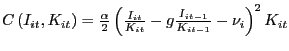$$C\left( {I_{it} ,K_{it} } \right) =\frac{\alpha}{2}\left( {\frac{I_{it} }{K_{it} }-g\frac{I_{it-1} }{K_{it-1} }-\nu_{i} } \right) ^{2}K_{it}$$ (A9)

It includes the lagged investment to capital ratio to capture strong persistence observed in the data. This can be explained by investment arrangements made by firms with costly cancellation costs. $\nu_{i}$ is a firm specific effect and $i$ indexes firms.⁴¹

MPK$_{it}$ is parameterized using a sales-based measure derived from the profit maximization problem assuming a Cobb-Douglas production function. It can be expressed as:⁴²

$$MPK_{it} =\theta_{i} \frac{S_{it} }{K_{it} }$$ (A10)

At the center of this estimation is the definition of the stochastic discount factor representing financing constraints Ô$_{t,t+s}$. The previous literature has relied on ad hoc parameterizations using observed characteristics of firms' financial health to identify the effect of financing constraints on investment decisions. This study follows Love (2003) and uses the "stock of liquid assets", namely the value of cash and equivalents, and divides it by the capital stock to parameterize Ô $_{i;t,t+s}$ as:

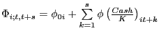$$\Phi_{i;t,t+s} =\phi_{0i} +\sum\limits_{k=1}^{s} {\phi\left( {\frac{Cash} {K}} \right) _{it+k} }$$ (A11)

Cash is measured at the beginning of period $t$ and $\phi_{0i}$ is a firm specific effect.

The main hypothesis of this paper is that financial integration reduces financing constraints. To test this, $\phi$ is allowed to vary with the states' ($j)$ measure of financial integration. So, Ô $_{i;t,t+s}$ is defined as:

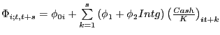$$\Phi_{i;t,t+s} =\phi_{0i} +\sum\limits_{k=1}^{s} {\left( {\phi_{1} +\phi_{2} Intg} \right) \left( {\frac{Cash}{K}} \right) _{it+k} }$$ (A12)

Then, (A12) is replaced in (A8) to obtain:

$$\begin{array}[c]{c} 1+\frac{\partial C\left( {I_{it} ,K_{it} } \right) }{\partial I_{it} }=\mathrm{Z}+E_{t} \left[ {\sum\limits_{s=1}^{\infty}{\beta^{s}\left( {1-\delta} \right) ^{s-1}MPK_{it+s} } } \right] \ +\varphi_{1} \phi E_{t} \left[ {\sum\limits_{s=1}^{\infty}{\sum \limits_{k=1}^{s} {\beta^{s}\left( {1-\delta} \right) ^{s-1}\left( {\frac{Cash}{K}} \right) _{it+k} } } } \right] \ +\varphi_{2} \phi E_{t} \left[ {\sum\limits_{s=1}^{\infty}{\sum \limits_{k=1}^{s} {\beta^{s}\left( {1-\delta} \right) ^{s-1}\left( {\frac{Cash}{K}\ast Intg} \right) _{it+k} } } } \right] \ \end{array}$$ (A13)

Then, MPK$_{it}$, $\left( {{Cash} \mathord{\left/ {\vphantom {{Cash} K}} \right. \kern-\nulldelimiterspace} K} \right) _{it}$ and $\left( {\left( {{Cash} \mathord{\left/ {\vphantom {{Cash} K}} \right. \kern-\nulldelimiterspace} K} \right) \ast Intg} \right) _{it}$ are assumed to be represented by a vector autoregressive process of order one. This characterization makes it possible to express (A13) as a linear function of the current value of the variables. This simplification coupled with the assumption of rational expectations, and equations (A9), (A10) and (A13), define the central estimating equation shown in (1).

Appendix 2

Sample Selection

Sample Selection: All observation in the Compustat North-America database provided by WRDS between 1976 and 1994.

Deletion Criteria:

• Firms located outside the U.S.


• All firms with no information on its location (state) and firms with changes the location of its headquarters within the sample period.


• All firms outside the manufacturing sector (SIC 2000-3999).


• Firms with missing data for I/K, Sales/K, Cash/K, and Real Assets.


• All firms located in South Dakota, Delaware and Puerto Rico.


• All firms with Assets <=0.


• All firms with Sales <=0.


• All firms with Capital <=0.


• All firms with Real Sales Growth <-100 or >100


• All firms with Sales/K <0, Cash/K <0 or I/K <0.


• All firms with Capital Stock Growth >100


• Top 1 and bottom 1 percentile of Sales/K and Cash/K.


• Firms with less than 2 years before and after interstate agreement.

Appendix 3

Variable Definitions

Compustat data items in parenthesis.

Variable	Acronym	Definition (Compustat Data Item)
Real Assets	-	Total assets at the beginning of the period (Compustat data item x6) adjusted using the GDP deflator.
Capital Stock	K	Net Property, Plant and Equipment. (x8)
Cash Stock	Cash/K	Cash plus equivalents (x1) scaled by capital.
Investment	I/K	Gross Investment scaled by Capital. (x30/x8(t-1))
Net Sales	Sales/K	Net sales at the end of period t-1 (x12). Scaled by capital.
Total Debt	-	Total debt is defined as Long Term Debt plus Current Liabilities (x9+x34)
Leverage	-	The ratio of total debt to total assets. ((x9+x34)/x6))
Tobin's Q	Tobin q	Market value plus book value of assets minus common equity and deferred taxes by the book value of assets. ((x6-x60-x74+x25*x199)/x6)
Short-term borrowing spread	-	Weighted average interest rate for short-term borrowing (x105) minus the prime rate.

Table I:  Year of Banking Deregulation and Share of Deposits Held by Multi-State Banks by State

The source for the deregulation dates is Berger, Kashyap, and Scalise (1995). The share of deposits is calculated using information from the Call Reports.

State	Interstate banking deregulation year	Average share of deposits 1976-1981	Average share of deposits 1982-1994	Share of total deposits in local MSBs minus share of total deposits in out-of-state MSBs (average after deregulation)
ALASKA	1982	0.00	0.15	-0.15
ALABAMA	1987	0.00	0.38	0.59
ARKANSAS	1989	0.00	0.11	0.19
ARIZONA	1986	0.28	0.69	-0.43
CALIFORNIA	1987	0.14	0.62	0.36
COLORADO	1988	0.04	0.21	-0.31
CONNECTICUT	1983	0.06	0.53	-0.08
DISTRICT OF COLUMBIA	1985	0.09	0.64	-0.19
FLORIDA	1985	0.01	0.49	-0.22
GEORGIA	1985	0.00	0.47	0.04
IOWA	1991	0.07	0.12	-0.22
IDAHO	1985	0.38	0.77	-0.11
ILLINOIS	1986	0.02	0.38	0.08
INDIANA	1986	0.00	0.27	-0.21
KANSAS	1992	0.00	0.06	0.07
KENTUCKY	1984	0.00	0.33	-0.09
LOUISIANA	1987	0.00	0.06	0.03
MASSACHUSETTS	1983	0.00	0.53	0.32
MARYLAND	1985	0.02	0.68	-0.03
MAINE	1978	0.00	0.67	-0.51
MICHIGAN	1986	0.02	0.53	0.67
MINNESOTA	1986	0.53	0.53	0.48
MISSOURI	1986	0.08	0.40	0.52
MISSISSIPPI	1988	0.00	0.20	0.28
MONTANA	1993	0.42	0.37	-0.29
NORTH CAROLINA	1985	0.04	0.61	0.71
NORTH DAKOTA	1991	0.32	0.31	-0.30
NEBRASKA	1990	0.08	0.18	0.06
NEW HAMPSHIRE	1987	0.00	0.17	-0.40
NEW JERSEY	1986	0.00	0.35	0.09
NEW MEXICO	1989	0.12	0.30	-0.04
NEVADA	1985	0.44	0.69	-0.60
NEW YORK	1982	0.15	0.91	0.51
OHIO	1985	0.00	0.46	0.51
OKLAHOMA	1987	0.00	0.05	-0.08
OREGON	1986	0.41	0.75	-0.07
PENNSYLVANIA	1986	0.00	0.51	0.43
RHODE ISLAND	1984	0.07	0.65	0.18
SOUTH CAROLINA	1986	0.00	0.36	-0.50
TENNESSEE	1985	0.02	0.34	-0.05
TEXAS	1987	0.00	0.29	-0.30
UTAH	1984	0.44	0.67	0.23
VIRGINIA	1985	0.05	0.50	0.31
VERMONT	1988	0.00	0.02	-0.02
WASHINGTON	1987	0.09	0.67	-0.71
WISCONSIN	1987	0.03	0.32	0.20
WEST VIRGINIA	1988	0.00	0.14	0.08
WYOMING	1987	0.14	0.26	-0.35
Total	-	0.09	0.41	-

Table II:  Sample Coverage for Firms by State

Firm level data is from Compustat North America. It includes publicly-traded firms in the manufacturing sector (SIC 2000-3999) from 1976 to 1994. Sample selection details are described in Appendix 2.

State	Number of firms	Pct. of total firms	Number of observations	Pct. of total observations	Average years per firm
ALABAMA	6	0.3%	89	0.3%	14.8
ARKANSAS	5	0.3%	82	0.3%	16.4
ARIZONA	10	0.6%	135	0.5%	13.5
CALIFORNIA	217	12.7%	2907	11.3%	13.4
COLORADO	27	1.6%	370	1.4%	13.7
CONNECTICUT	95	5.5%	1374	5.4%	14.5
DISTRICT OF COLUMBIA	1	0.1%	19	0.1%	19.0
FLORIDA	58	3.4%	841	3.3%	14.5
GEORGIA	26	1.5%	436	1.7%	16.8
IOWA	12	0.7%	199	0.8%	16.6
IDAHO	1	0.1%	17	0.1%	17.0
ILLINOIS	107	6.2%	1701	6.6%	15.9
INDIANA	33	1.9%	527	2.1%	16.0
KANSAS	10	0.6%	134	0.5%	13.4
KENTUCKY	6	0.3%	93	0.4%	15.5
LOUISIANA	5	0.3%	84	0.3%	16.8
MASSACHUSETTS	89	5.2%	1318	5.1%	14.8
MARYLAND	23	1.3%	345	1.3%	15.0
MAINE	4	0.2%	53	0.2%	13.3
MICHIGAN	63	3.7%	1051	4.1%	16.7
MINNESOTA	71	4.1%	1047	4.1%	14.7
MISSOURI	35	2.0%	580	2.3%	16.6
MISSISSIPPI	2	0.1%	37	0.1%	18.5
NORTH CAROLINA	34	2.0%	538	2.1%	15.8
NEBRASKA	5	0.3%	66	0.3%	13.2
NEW HAMPSHIRE	8	0.5%	116	0.5%	14.5
NEW JERSEY	113	6.6%	1667	6.5%	14.8
NEW MEXICO	2	0.1%	32	0.1%	16.0
NEVADA	2	0.1%	25	0.1%	12.5
NEW YORK	236	13.8%	3335	13.0%	14.1
OHIO	85	5.0%	1402	5.5%	16.5
OKLAHOMA	9	0.5%	129	0.5%	14.3
OREGON	16	0.9%	242	0.9%	15.1
PENNSYLVANIA	94	5.5%	1540	6.0%	16.4
RHODE ISLAND	11	0.6%	158	0.6%	14.4
SOUTH CAROLINA	7	0.4%	100	0.4%	14.3
TENNESSEE	9	0.5%	147	0.6%	16.3
TEXAS	79	4.6%	1164	4.5%	14.7
UTAH	8	0.5%	104	0.4%	13.0
VIRGINIA	34	2.0%	560	2.2%	16.5
VERMONT	1	0.1%	19	0.1%	19.0
WASHINGTON	20	1.2%	285	1.1%	14.3
WISCONSIN	35	2.0%	584	2.3%	16.7
WEST VIRGINIA	1	0.1%	15	0.1%	15.0
Total	1,715	-	25,667	-	15.0

Table III:  Summary Statistics for Firms

Firm level data is from Compustat North America. It includes publicly-traded firms in the U.S. manufacturing sector (SIC 2000-3999) from 1976 to 1994. Sample selection details are described in Appendix 2. Real assets is defined in millions of 1995 U.S. dollars. $K$ is the stock of net property, plant, and equipment, and $I$ is the yearly expenditures on these assets. Cash is defined as the firm's stock of cash and short-term investments. Total Debt is equal to long-term debt plus current liabilities. The Short-term Interest Rate Spread is defined as the firms' average interest rate on short-term loans in the fiscal year minus the prime rate. In Panels B and C, firms are classified as having access to public debt markets if they issued or had rated commercial paper or bonds between 1970 and 1994.

Table III:  Summary Statistics for Firms: Panel A - Full Sample

Statistic	Real Assets	I/K	Sales/K	Cash/K	Total Debt/    Assets	Short-term Interest Rate Spread
Mean	1424.0	0.3	6.4	0.5	0.3	0.7
Median	111.5	0.2	4.9	0.2	0.2	0.2
Maximum	223844.8	2.8	54.8	12.7	10.2	18.1
Minimum	0.06	0.0	0.2	0.0	0.0	-10.7
Std. Dev.	6370.6	0.2	5.7	1.0	0.3	2.8
Observations	25667	25667	25667	25667	25642	7051

Table III:  Summary Statistics for Firms: Panel B - Firms without Access to Public Debt Markets

Statistic	Real Assets	I/K	Sales/K	Cash/K	Total Debt / Assets	Short-term Interest Rate Spread
Mean	470.2	0.3	7.3	0.6	0.2	0.6
Median	43.5	0.2	5.5	0.2	0.2	0.3
Maximum	129342.3	2.3	54.8	12.7	10.2	17.1
Minimum	0.1	0.0	0.2	0.0	0.0	-10.7
Std. Dev.	4178.8	0.2	6.3	1.1	0.3	2.3
Observations	16220	16220	16220	16220	16196	4044

Table III:  Summary Statistics for Firms: Panel C - Firms with Access to Public Debt Markets

Statistic	Real Assets	I/K	Sales/K	Cash/K	Total Debt/    Assets	Short-term Interest Rate Spread
Mean	3061.6	0.3	5.0	0.4	0.3	0.7
Median	793.3	0.2	4.0	0.2	0.2	-0.1
Maximum	223844.8	2.8	53.1	12.3	4.1	18.1
Minimum	0.4	0.0	0.2	0.0	0.0	-8.7
Std. Dev.	8720.3	0.2	4.1	0.8	0.2	3.3
Observations	9447	9447	9447	9447	9446	2966

Table IV:  Bank Integration and Financial Constraints

The results are from the following equation estimated using System GMM:

$$\frac{I_{it} }{K_{it-1} }=\alpha_{0} +\alpha_{1} \frac{I_{it-1} }{K_{it-2} }+\alpha_{2} \frac{Sales_{it-1} }{K_{it-1} }+\alpha_{3} \frac{Cash_{it-1} }{K_{it-1} }+\alpha_{4} \frac{Cash_{it-1} }{K_{it-1} }\times Intg_{jt} +\alpha_{5} Intg_{jt} +\beta Z_{jt} +f_{i} +h_{t} +\varepsilon_{it}$$

$I_{t}/K_{t-1}$ is the ratio of investment in the current period to capital at the beginning of the period. $S_{ t-1}/K_{ t-1}$ and Cash $_{t-1}/K_{t-1}$ are the ratios of sales and the stock of cash and equivalents to capital at the beginning of the period. $Z_{jt}$ is the growth in real per capita income by state. Columns (1) through (4) differ in the definition of Intg, the variable that measures bank integration. In column (1), Intg is a dummy variable equal to one if the state passed a law allowing interstate banking. In column (2), Intg is the share of deposits in Multi-State banks (MSBs) by state and year. An MSB is an institution with subsidiaries in at least two different states. In column (3) Intg is the share of commercial and industrial loans (C&I) held in MSBs. In column (4) Intg is the share of assets in MSBs by state and year. Lags 3 and 4 of endogenous and predetermined variables and industry dummies (2-digit SIC) are used as instruments. Hansen test is the p-value of the J-statistic for over-identifying restrictions (distributed chi-square). The AR 1 (2) test shows the p-value from Arellano and Bond's (1991) first (second) order autocorrelation test. Windmeijer (2005) corrected standard errors shown in brackets.

Intg measured as:	Interstate Agreement (1)	Share of Deposits (2)	Share of C&I (3)	Share of  Assets (4)
It-1/Kt-2	0.255***	0.261***	0.260***	0.261***
std. error	[0.039]	[0.041]	[0.040]	[0.040]
Salest-1/Kt-1	0.007***	0.007***	0.007***	0.007***
std. error	[0.001]	[0.001]	[0.001]	[0.001]
Casht-1/Kt-1	0.023**	0.025*	0.025*	0.024*
std. error	[0.011]	[0.013]	[0.013]	[0.014]
(Casht-1/Kt-1) x Intgjt	-0.019*	-0.031	-0.027	-0.028
std. error	[0.011]	[0.022]	[0.020]	[0.022]
Intgjt	0.006	0.027	0.021	0.022
std. error	[0.012]	[0.037]	[0.035]	[0.037]
Observations	23078	23078	23078	23078
Number of Firms	1715	1715	1715	1715
Hansen test	0.30	0.30	0.29	0.30
AR 1 test	0	0	0	0
AR 2 test	0.94	0.89	0.89	0.88

Standard errors in brackets.
*  significant at 10%; **  significant at 5%; ***  significant at 1%.

Table V:  Bank Integration, Financial Constraints, and Access to the Public Debt Market

The results are from the following equation estimated using System GMM:

$$\frac{I_{it} }{K_{it-1} }=\alpha_{0} +\alpha_{1} \frac{I_{it-1} }{K_{it-2} }+\alpha_{2} \frac{Sales_{it-1} }{K_{it-1} }+\alpha_{3} \frac{Cash_{it-1} }{K_{it-1} }+\alpha_{4} \frac{Cash_{it-1} }{K_{it-1} }\times Intg_{jt} +\alpha_{5} Intg_{jt} +\beta Z_{jt} +f_{i} +h_{t} +\varepsilon_{it}$$

I_t/K_t-1 is the ratio of investment in the current period to capital at the beginning of the period. S_t-1/K_t-1 and Cash_t-1/K_t-1 are the ratios of sales and the stock of cash and equivalents to capital at the beginning of the period. Z_jt is the growth in real per capita income by state. Columns (1) through (4) differ in the definition of Intg, the variable that measures bank integration, and the degree of firms' bank dependence proxied by access to the public debt market. In columns (1) and (2), Intg is a dummy variable equal to one if the state passed a law allowing interstate banking. In column (3) and (4), Intg is the share of deposits in Multi-State banks (MSBs) by state and year. An MSB is an institution with subsidiaries in at least two different states. Firms included in the estimation of columns (1) and (3) did not have any commercial paper or bond issues (or ratings) between 1970 and 1994, and had average positive total debt holdings in this period. The complement of this group is included in the estimations of columns (2) and (4). Lags 3 and 4 of endogenous and predetermined variables and industry dummies (2-digit SIC) are used as instruments. Hansen test is the p-value of the J-statistic for over-identifying restrictions (distributed chi-square). The AR 1 (2) test shows the p-value from Arellano and Bond's (1991) first (second) order autocorrelation test. Windmeijer (2005) corrected standard errors shown in brackets.

Intg measured as:	Interstate Agreement	Interstate Agreement	Share of Deposits	Share of Deposits
Bank Dependence (Access to public debt market):	Bank-Dependent (1)	Not Bank-Dependent (2)	Bank-Dependent (3)	Not Bank-Dependent (4)
It-1/Kt-2	0.217***	0.333***	0.217***	0.324***
std. error	[0.042]	[0.068]	[0.045]	[0.066]
Salest-1/Kt-1	0.008***	0.004*	0.008***	0.004*
std. error	[0.001]	[0.002]	[0.001]	[0.002]
Casht-1/Kt-1	0.029**	0.023	0.038***	0.013
std. error	[0.011]	[0.016]	[0.014]	[0.015]
(Casht-1/Kt-1) x Intgjt	-0.032***	0.003	-0.063**	0.025
std. error	[0.012]	[0.018]	[0.025]	[0.021]
Intgjt	0.011	-0.007	0.049	-0.088
std. error	[0.016]	[0.020]	[0.041]	[0.054]
Observations	14428	8650	14428	8650
Number of Firms	1140	575	1140	575
Hansen test	0.67	0.01	0.72	0.02
AR 1 test	0	0	0	0
AR 2 test	0.31	0.11	0.29	0.11

Standard errors in brackets.
*  significant at 10%; **  significant at 5%; ***  significant at 1%.

Table VI:  Bank Integration, Financial Constraints, and Firm Size

The results are from the following equation estimated using System GMM:

$$\frac{I_{it} }{K_{it-1} }=\alpha_{0} +\alpha_{1} \frac{I_{it-1} }{K_{it-2} }+\alpha_{2} \frac{Sales_{it-1} }{K_{it-1} }+\alpha_{3} \frac{Cash_{it-1} }{K_{it-1} }+\alpha_{4} \frac{Cash_{it-1} }{K_{it-1} }\times Intg_{jt} +\alpha_{5} Intg_{jt} +\beta Z_{jt} +f_{i} +h_{t} +\varepsilon_{it}$$

$I_{t}/K_{t-1}$ is the ratio of investment in the current period to capital at the beginning of the period. $S_{ t-1}/K_{ t-1}$ and Cash $_{t-1}/K_{t-1}$ are the ratios of sales and the stock of cash and equivalents to capital at the beginning of the period. $Z_{jt}$ is the growth in real per capita income by state. Columns (1) through (8) differ in the definition of Intg, the variable that measures bank integration, and the degree of firms' bank dependence proxied by the firms' size measured in terms of real assets (in 1995 U.S. dollars). In columns (1) through (4), Intg is a dummy variable equal to one if the state passed a law allowing interstate banking. In column (5) through (8), Intg is the share of deposits in Multi-State banks (MSBs) by state and year. An MSB is an institution with subsidiaries in at least two different states. Firms included in the estimation of columns (1) and (5) have real assets below the sample median (computed by State). The complement of this group is included in the estimations of columns (2) and (6). Firms included in the estimation of columns (6>) and (7) are in the bottom tercile of the real assets distribution, while firms in (4) and (8) are in the top tercile. Lags 3 and 4 of endogenous and predetermined variables and industry dummies (2-digit SIC) are used as instruments. Hansen test is the p-value of the J-statistic for over-identifying restrictions (distributed chi-square). The AR 1 (2) test shows the p-value from Arellano and Bond's (1991) first (second) order autocorrelation test. Windmeijer (2005) corrected standard errors shown in brackets.

Intg measured as:	Interstate Agreement	Interstate Agreement	Interstate Agreement	Interstate Agreement	Share of Deposits	Share of Deposits	Share of Deposits	Share of Deposits
Bank Dependence (Firm Size - Assets):	Less than Median by State (1)	More than Median by State (2)	Bottom Tercile (3)	Top Tercile (4)	Less than Median by State (5)	More than Median by State (6)	Bottom Tercile (7)	Top Tercile (8)
It-1/Kt-2	0.137***	0.348***	0.091	0.324***	0.140***	0.357***	0.097*	0.318***
t-stat	[0.052]	[0.044]	[0.058]	[0.044]	[0.054]	[0.045]	[0.058]	[0.044]
Salest-1/Kt-1	0.008***	0.007***	0.007***	0.008**	0.008***	0.007***	0.007***	0.009**
t-stat	[0.002]	[0.002]	[0.002]	[0.003]	[0.002]	[0.002]	[0.002]	[0.003]
Casht-1/Kt-1	0.036***	0.049***	0.038***	0.063***	0.041***	0.052**	0.036**	0.089***
t-stat	[0.012]	[0.018]	[0.013]	[0.024]	[0.014]	[0.025]	[0.015]	[0.027]
(Casht-1/Kt-1) x Intgjt	-0.037***	-0.015	-0.044***	-0.009	-0.067***	-0.029	-0.065**	-0.062
t-stat	[0.012]	[0.019]	[0.013]	[0.024]	[0.023]	[0.039]	[0.029]	[0.047]
Intgjt	0.042**	-0.009	0.046**	-0.006	0.123***	-0.011	0.092	0.009
t-stat	[0.017]	[0.014]	[0.022]	[0.017]	[0.044]	[0.036]	[0.062]	[0.034]
Observations	11307	11771	7418	7884	11307	11771	7418	7884
Number of Firms	1136	985	851	645	1136	985	851	645
Hansen test	0.13	0.03	0.26	0.02	0.19	0.04	0.24	0.04
AR 1 test	0	0	0	0	0	0	0	0
AR 2 test	0.14	0.12	0.11	0.88	0.14	0.11	0.11	0.88

Standard errors in brackets.
*  significant at 10%; **  significant at 5%; ***  significant at 1%.

Table VII:  Banking Exporters, Importers, and Firm Financial Constraints

The results are from the following equation estimated using System GMM:

$$\frac{I_{it} }{K_{it-1} }=\alpha_{0} +\alpha_{1} \frac{I_{it-1} }{K_{it-2} }+\alpha_{2} \frac{Sales_{it-1} }{K_{it-1} }+\alpha_{3} \frac{Cash_{it-1} }{K_{it-1} }+\alpha_{4} \frac{Cash_{it-1} }{K_{it-1} }\times Intg_{jt} +\alpha_{5} Intg_{jt} +\beta Z_{jt} +f_{i} +h_{t} +\varepsilon_{it}$$

$I_{t}/K_{t-1}$ is the ratio of investment in the current period to capital at the beginning of the period. $S_{ t-1}/K_{ t-1}$ and Cash $_{t-1}/K_{t-1}$ are the ratios of sales and the stock of cash and equivalents to capital at the beginning of the period. $Z_{jt}$ is the growth in real per capita income by state. Columns (1) through (6) differ in the definition of bank integration, the variable that measures bank integration, and the degree of firms' bank dependence. In columns (1), (3), and (5), the Share of Banking Exporters is the share of deposits in locally headquartered Multi-State banks (MSBs) by state and year. An MSB is an institution with subsidiaries in at least two different states. The Share of Banking Importers is the fraction of deposits held in out-of-state MSBs in the host state. In columns (2), (4), and (6) the same bank integration measure is computed, but using the share of Commercial and Industrial (C&I) loans instead of deposits. Firms included in the estimation of columns (1) and (2) did not have any commercial paper or bond issues (or ratings) between 1970 and 1994, and had average positive total debt holdings in this period. Firms included in the estimations of columns (3) through (6) are defined as small in terms of their stock of real assets (in 1995 U.S. dollars). Lags 3 and 4 of endogenous and predetermined variables and industry dummies (2-digit SIC) are used as instruments. Hansen test is the p-value of the J-statistic for over-identifying restrictions (distributed chi-square). The AR 1 (2) test shows the p-value from Arellano and Bond's (1991) first (second) order autocorrelation test. Windmeijer (2005) corrected standard errors shown in brackets.

Bank Dependence:	No access to public debt market	No access to public debt market	Firm Size: Assets are less than the Median by State	Firm Size: Assets are less than the Median by State	Firm Size: Assets are in the Bottom Tercile	Firm Size: Assets are in the Bottom Tercile
Bank Integration in terms of:	Deposits (1)	C & I Loans (2)	Deposits (3)	C & I Loans (4)	Deposits (5)	C & I Loans (6)
It-1/Kt-2	0.207***	0.210***	0.132**	0.133**	0.104*	0.102
t-stat	[0.044]	[0.044]	[0.053]	[0.053]	[0.061]	[0.062]
Salest-1/Kt-1	0.008***	0.008***	0.007***	0.007***	0.006***	0.006***
t-stat	[0.001]	[0.001]	[0.002]	[0.002]	[0.002]	[0.002]
Casht-1/Kt-1	0.039***	0.038**	0.041***	0.043***	0.034**	0.034**
t-stat	[0.014]	[0.015]	[0.014]	[0.015]	[0.016]	[0.017]
(Casht-1/Kt-1) x Share of Banking Exportersjt	-0.080***	-0.070***	-0.074***	-0.068***	-0.087**	-0.078***
t-stat	[0.029]	[0.025]	[0.028]	[0.024]	[0.036]	[0.030]
(Casht-1/Kt-1) x Share of Banking Importersjt	-0.019	-0.01	-0.045	-0.036	0.011	0.027
t-stat	[0.050]	[0.045]	[0.055]	[0.051]	[0.079]	[0.070]
Share of Banking Exportersjt	0.078	0.066	0.112	0.121**	0.112	0.115
t-stat	[0.057]	[0.047]	[0.073]	[0.061]	[0.083]	[0.071]
Share of Banking Importersjt	-0.052	-0.064	0.135	0.088	0.028	-0.06
t-stat	[0.136]	[0.127]	[0.147]	[0.136]	[0.191]	[0.178]
Observations	14425	14425	11306	11306	7417	7417
Number of Firms	1140	1140	1136	1136	851	851
Hansen test	0.79	0.79	0.31	0.31	0.22	0.23
AR 1 test	0	0	0	0	0	0
AR 2 test	0.23	0.26	0.11	0.11	0.15	0.15

Standard errors in brackets.
*  significant at 10%; **  significant at 5%; ***  significant at 1%.

Table VIII  Sensitivity Analysis-Different Controls and Variable Definitions

The results are from the following equation estimated using System GMM:

$$\frac{I_{it} }{K_{it-1} }=\alpha_{0} +\alpha_{1} \frac{I_{it-1} }{K_{it-2} }+\alpha_{2} MPK_{t-1} +\alpha_{3} \frac{Cash_{it-1} }{K_{it-1} }+\alpha_{4} \frac{Cash_{it-1} }{K_{it-1} }\times Intg_{jt} +\alpha_{5} Intg_{jt} +\beta Z_{jt} +f_{i} +h_{t} +\varepsilon_{it}$$

$I_{t}/K_{t-1}$ is the ratio of investment in the current period to capital at the beginning of the period. $S_{ t-1}/K_{ t-1}$ and Cash $_{t-1}/K_{t-1}$ are the ratios of sales and the stock of cash and equivalents to capital at the beginning of the period. $Z_{jt}$ is the growth in real per capita income by state. Firms included in the estimations did not have any commercial paper or bond issues (or ratings) between 1970 and 1994, and had average positive total debt holdings in this period. Columns (1) through (6) differ in the definition of Intg (the variable that measures bank integration), the definition of some variables, and the inclusion of new controls. In columns (1), (3), and (5), Intg is a dummy variable equal to one if the state passed a law allowing interstate banking. In column (2), (4), and (6), Intg is the share of deposits in Multi-State banks (MSBs) by state and year. An MSB is an institution with subsidiaries in at least two different states. Bank Concentration is a dummy equal to one if the Herfindahl-Hirshman Index (HHI) for deposits is below the median. Leverage is the ratio of total debt to assets. Tobin q is a proxy for the marginal profitability of capital (MPK). Lags 3 and 4 of endogenous and predetermined variables and industry dummies (2-digit SIC) are used as instruments. Hansen test is the p-value of the J-statistic for over-identifying restrictions (distributed chi-square). The AR 1 (2) test shows the p-value from Arellano and Bond's (1991) first (second) order autocorrelation test. Windmeijer (2005) corrected standard errors shown in brackets.

Added or changed variables:	Bank Concentration	Bank Concentration	Leverage	Leverage	Tobin's Q	Tobin's Q
Intg measured as:	Interstate Agreement (1)	Share of Deposits (2)	Interstate Agreement (3)	Share of Deposits (4)	Interstate Agreement (5)	Share of Deposits (6)
It-1/Kt-2	0.215***	0.208***	0.283***	0.289***	0.210***	0.218***
t-stat	[0.039]	[0.042]	[0.045]	[0.047]	[0.044]	[0.045]
Salest-1/Kt-1	0.008***	0.008***	0.008***	0.008***	-	-
t-stat	[0.001]	[0.001]	[0.001]	[0.001]	-	-
Casht-1/Kt-1	0.035***	0.032**	0.019	0.033**	0.033***	0.048***
t-stat	[0.012]	[0.013]	[0.012]	[0.015]	[0.012]	[0.018]
(Casht-1/Kt-1) x Intgjt	-0.029**	-0.042*	-0.028**	-0.068***	-0.026**	-0.069**
t-stat	[0.011]	[0.022]	[0.012]	[0.025]	[0.012]	[0.028]
(Casht-1/Kt-1) x Bank Concentrationjt	-0.005	0.001	-	-	-	-
t-stat	[0.013]	[0.013]	-	-	-	-
Leveraget-1	-	-	-0.117**	-0.115**	-	-
t-stat	-	-	[0.054]	[0.055]	-	-
Tobin q t-1	-	-	-	-	0.039***	0.038***
t-stat	-	-	-	-	[0.009]	[0.009]
Observations	14425	14425	14407	14407	11131	11131
Number of Firms	1140	1140	1140	1140	900	900
Hansen test	0.71	0.72	0.46	0.56	0.74	0.74
AR 1 test	0	0	0	0	0	0
AR 2 test	0.28	0.24	0.99	0.99	0.17	0.18

Standard errors in brackets.
*  significant at 10%; **  significant at 5%; ***  significant at 1%.

Table IX:  Sensitivity Analysis-Sample Selection

The results are from the following equation estimated using System GMM:

$$\frac{I_{it} }{K_{it-1} }=\alpha_{0} +\alpha_{1} \frac{I_{it-1} }{K_{it-2} }+\alpha_{2} \frac{Sales_{it-1} }{K_{it-1} }+\alpha_{3} \frac{Cash_{it-1} }{K_{it-1} }+\alpha_{4} \frac{Cash_{it-1} }{K_{it-1} }\times Intg_{jt} +\alpha_{5} Intg_{jt} +\beta Z_{jt} +f_{i} +h_{t} +\varepsilon_{it}$$

$I_{t}/K_{t-1}$ is the ratio of investment in the current period to capital at the beginning of the period. $S_{ t-1}/K_{ t-1}$ and Cash $_{t-1}/K_{t-1}$ are the ratios of sales and the stock of cash and equivalents to capital at the beginning of the period. $Z_{jt}$ is the growth in real per capita income by state. Firms included in the estimations did not have any commercial paper or bond issues (or ratings) between 1970 and 1994, and had average positive total debt holdings in this period. Columns (1) through (6) differ in the definition of Intg (the variable that measures bank integration), and the sample of firms included. In columns (1), (3), and (5), Intg is a dummy variable equal to one if the state passed a law allowing interstate banking. In column (2), (4), and (6), Intg is the share of deposits in Multi-State banks (MSBs) by state and year. An MSB is an institution with subsidiaries in at least two different states. Modified sample restrictions are describe in the first row. Lags 3 and 4 of endogenous and predetermined variables and industry dummies (2-digit SIC) are used as instruments. Hansen test is the p-value of the J-statistic for over-identifying restrictions (distributed chi-square). The AR 1 (2) test shows the p-value from Arellano and Bond's (1991) first (second) order autocorrelation test. Windmeijer (2005) corrected standard errors shown in brackets.

Sample restriction:	Exclude states with simultaneous intrastate branching deregulation	Exclude states with simultaneous intrastate branching deregulation	Exclude firms located in California and New York	Exclude firms located in California and New York	Include firms with obs. for at least 4 consecutive years	Include firms with obs. for at least 4 consecutive years
Intg measured as:	Interstate Agreement (1)	Share of Deposits (2)	Interstate Agreement (3)	Share of Deposits (4)	Interstate Agreement (5)	Share of Deposits (6)
It-1/Kt-2	0.235***	0.236***	0.204***	0.211***	0.250***	0.243***
t-stat	[0.045]	[0.049]	[0.053]	[0.058]	[0.046]	[0.050]
Salest-1/Kt-1	0.007***	0.007***	0.009***	0.009***	0.007***	0.007***
t-stat	[0.001]	[0.001]	[0.002]	[0.002]	[0.001]	[0.001]
Casht-1/Kt-1	0.032**	0.035**	0.030**	0.029**	0.035***	0.041***
t-stat	[0.013]	[0.016]	[0.013]	[0.013]	[0.011]	[0.013]
(Casht-1/Kt-1) x Intgjt	-0.032**	-0.047*	-0.035***	-0.062***	-0.021*	-0.039*
t-stat	[0.014]	[0.027]	[0.013]	[0.023]	[0.013]	[0.022]
Intgjt	0.008	0.044	0.014	0.049	0.001	0.005
t-stat	[0.017]	[0.044]	[0.019]	[0.055]	[0.016]	[0.042]
Observations	11993	11993	10847	10847	21938	21938
Number of Firms	953	953	829	829	2488	2488
Hansen test	0.46	0.45	0.51	0.57	0.17	0.17
AR 1 test	0	0	0	0	0	0
AR 2 test	0.74	0.74	0.48	0.58	0.84	0.76

Standard errors in brackets.
*  significant at 10%; **  significant at 5%; ***  significant at 1%.

Table X:  Bank Integration and Firms' Short-Term Borrowing Costs

The results are from the following equation estimated using the within estimator:

$$y_{it} =\beta_{0} +\beta_{1} Intg_{jt} +\sum\limits_{h=1}^{k} {\gamma_{h} Bank\,Dependence_{it}^{h} } +\sum\limits_{h=1}^{k} {\pi_{h} \left( {Bank\,Dependence_{it}^{h} \ast Intg_{jt} } \right) } +\delta X_{it} +\beta Z_{jt} +\eta_{i} +\mu_{t} +\varepsilon_{it}$$

The dependent variable is the spread between the firms' average interest rate for short-term borrowing and the prime rate. Intg is a dummy variable equal to one if the state passed a law allowing interstate banking. Bank Dependence is proxied by the firms' access to public debt markets and the firms' size. Public debt is an indicator variable equaling one if a firm did not have any commercial paper or bond issues (or ratings) between 1970 and 1994, and had average positive total debt holdings in this period. Small and Large are dummy variables equal to one if the value of the firm's lagged real assets is located in the bottom tercile or top tercile, respectively. $X_{it}$ are additional firm controls including the lagged log of real assets and EBITDA and tangible assets divided by total assets. $Z_{jt}$ includes the log of the Herfindahl-Hirshman Index (HHI) for bank deposits at the state level and the growth in real per capita income. Robust standard errors (in brackets) are clustered by state and year.

Intg measured as:	Interstate Agreement	Interstate Agreement	Interstate Agreement	Interstate Agreement	Share of Deposits	Share of Deposits	Share of Deposits	Share of Deposits
Bank Dependence proxy:	Access to public debt market (1)	Access to public debt market (2)	Firm Size (3)	Firm Size (4)	Access to public debt market (5)	Access to public debt market (6)	Firm Size (7)	Firm Size (8)
Intgjt	0.211	0.242	0.036	0.038	-0.147	-0.087	-0.664***	-0.663***
t-stat	[0.147]	[0.148]	[0.124]	[0.124]	[0.265]	[0.265]	[0.195]	[0.196]
Intgjt x Public Debti	-0.256*	-0.310**	-	-	-0.619**	-0.738***	-	-
t-stat	[0.131]	[0.134]	-	-	[0.276]	[0.279]	-	-
Smallt-1	-	-	0.168	-0.068	-	-	0.113	-0.116
t-stat	-	-	[0.137]	[0.133]	-	-	[0.157]	[0.155]
Larget-1	-	-	-0.475**	-0.239	-	-	-0.521**	-0.282
t-stat	-	-	[0.184]	[0.200]	-	-	[0.206]	[0.219]
Intgjt x Smallt-1	-	-	-0.249**	-0.240**	-	-	-0.193	-0.202
t-stat	-	-	[0.115]	[0.114]	-	-	[0.222]	[0.221]
Intgjt x Larget-1	-	-	0.261	0.241	-	-	0.57	0.531
t-stat	-	-	[0.176]	[0.177]	-	-	[0.361]	[0.363]
Additional Firm Controls	No	Yes	No	Yes	No	Yes	No	Yes
Observations	7034	6995	7051	7012	7034	6995	7051	7012
Number of Firms	831	829	835	833	831	829	835	833
R-squared	0.09	0.10	0.09	0.10	0.09	0.10	0.09	0.10

Robust standard errors clustered by state-year in brackets.
*  significant at 10%; **  significant at 5%; ***  significant at 1%.

Figure 1:  Average share of Multi-State banks in total banking activity.

The figure shows three measures of the degree of bank integration across states. The share of deposits (solid dark line) is the unweighted average share of deposits held in Multi-State banks (MSBs) in 47 states (excludes Delaware, Hawaii, and South Dakota) and the District of Columbia. An MSB is an institution with subsidiaries in at least two different states. Before 1994 information on the level of deposits is from the Call Reports, and after this year, from the FDIC's Summary of Deposits (solid light line). The two additional measures, the share of assets (discontinuous line) and of Commercial and Industrial (C&I) loans (dotted line) are constructed in the same way using Call Report information. Three vertical lines denote benchmarks in the process of bank integration: the first state to pass a law allowing out-of-state banks to acquire banks within its borders if the state of the acquiring bank reciprocates (Maine), the first states to reciprocate (Alaska and New York), and the year the Riegle-Neal Interstate Banking and Branching Efficiency Act was passed.

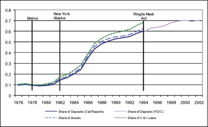
Data for Figure 1

Year	Share of Deposits (Call Reports)	Share of Assets	Share of C&I Loans	Share of Deposits (FDIC)
1976	0.0948693	0.0967	0.105362	-
1977	0.1001665	0.1025126	0.111035	-
1978	0.0936686	0.0963625	0.1028695	-
1979	0.0880857	0.0907886	0.0948486	-
1980	0.0922576	0.0988516	0.1074378	-
1981	0.1003195	0.1093908	0.1190431	-
1982	0.1439524	0.1539727	0.1743281	-
1983	0.1659135	0.1751137	0.1958356	-
1984	0.2008839	0.2123659	0.2364135	-
1985	0.2433627	0.2582925	0.2841429	-
1986	0.3482655	0.3712977	0.3921678	-
1987	0.4357436	0.4594417	0.4857315	-
1988	0.4822985	0.5067072	0.5363829	-
1989	0.5104819	0.5328171	0.5669128	-
1990	0.5295681	0.5478091	0.5874925	-
1991	0.5369498	0.5541974	0.5983449	-
1992	0.5523037	0.5714036	0.6185768	-
1993	0.5798324	0.5996663	0.6550658	-
1994	0.6027446	0.6253468	0.6834394	0.590981
1995	-	-	-	0.62919
1996	-	-	-	0.640033
1997	-	-	-	0.651036
1998	-	-	-	0.679633
1999	-	-	-	0.696106
2000	-	-	-	0.70221
2001	-	-	-	0.693692
2002	-	-	-	0.702233

Footnotes

*  Staff economist of the Division of International Finance of the Federal Reserve Board. I am indebted to Charles Calomiris for his encouragement, guidance, and very helpful discussions. I am also grateful to Stefania Albanesi, Ann Bartel, Allen Berger, Jose Berrospide, Janet Currie, Brendan O'Flaherty, Dale Henderson, Daniel Paravisini, Bruce Preston, Juan A. Robalino, Sanket Mohapatra, Bernard Salanié, and Gustavo Suarez. I would like to thank seminar participants at the Federal Reserve Bank of Boston, Columbia University, FDIC, Haverford College, Federal Reserve Board, and the OCC for valuable comments and discussions. The usual disclaimer applies. The authors' views do not necessarily reflect those of the Board of Governors of the Federal Reserve or the Federal Reserve System. Contact information: [email protected], (202) 452-2213. Return to text

1.  For a summary of these findings see Strahan (2003). Return to text

2.  Berger, Kashyap, and Scalise (1995) summarize the chronology of other regulatory changes that took place in the same period concerning bank deposits and capital requirements. Return to text

3.  In the most complete dataset, Houston and James (1996) collect data on bank debt for a random sample of 250 publicly-traded firms. It includes detailed information for their sampled firms in fiscal years 1980, 1985, and 1990. Return to text

4.  For a review of the literature see Hubbard (1998) and Schiantarelli (1996). Return to text

5.  Montana and Texas opted out. Return to text

6.  Hadlock, Houston, and Ryngaert (1999) find that acquisitions usually result in the replacement of the target's management. Berger, Demsetz, and Strahan (1999) summarize the main empirical facts linked to the consolidation of the U.S. banking industry. Return to text

7.  The authors also find that the sensitivity of investment to cash flow decreases in the first year after the firms' bank(s) is (are) involved in an M&A deal. Return to text

8.  This method was introduced in Fazzari, Hubbard, and Peterson (1988). For a review of the literature see Hubbard (1998) and Schiantarelli (1996). Return to text

9.  An explicit derivation of the model can be found in Appendix 1. Return to text

10.  Opler et al. (1999) find evidence for the precautionary motive of holding cash. Firms accumulate cash to insure against adverse shocks when access to capital markets is costly. This is particularly relevant for riskier firms. In related work, Almeida, Campello, and Weisbach (2004) show that financially constrained firms have a propensity to save cash out of cash flow. This pattern is not observed for unconstrained firms. Return to text

11.  The criticism on theoretical grounds can be found in Alti (2003), Cooper and Ejarque (2001), Gomes (2001), Kaplan and Zingales (1997, 2000), and Moyen (1994). The empirical findings are questioned by Cleary (1999), Erickson and Whited (2000), and Cleary, Povel, and Raith (2007). Return to text

12.  An alternative method to remove fixed effects is by forward-mean differencing the variables. This technique is commonly referred to as the Helmert's procedure. It removes only the forward mean, which has the advantage of preserving orthogonality between transformed errors and untransformed original variables. Results shown in the main estimations are robust to using this method. Return to text

13.  This estimator was proposed by Arellano and Bover (1995) and Blundell and Bond (1998). I implement it using the command xtabond2 in Stata, see Roodman (2006). Return to text

14.  This is equivalent to the assumption of predetermined regressors instead of strictly exogenous. Return to text

15.  The source for these dates is Berger, Kashyap, and Scalise (1995). Return to text

16.  Delaware and South Dakota are dropped from the sample due to the significant presence of credit card companies in these states starting in the 1980s. Hawaii did not deregulate before the Riegle-Neal act was passed in 1994. The District of Columbia is included in the sample. Return to text

17.  The Herfindahl-Hirschman Index is constructed as the sum of squared market shares for deposits in all banks by geographical market. It could range from 10,000 for highly concentrated markets to 0 for very competitive markets. Metropolitan Statistical Areas (MSAs) and counties are usually used as the definition for a market. In this analysis, a state will be defined as the market. Return to text

18.  Compustat North America is a database of U.S. and Canadian firms produced by Standard and Poor's investment services and includes fundamental and market information on more than 24,000 active and inactive publicly-held companies. Return to text

19.  The earliest year for which I have location information comes after the first bank entry deregulation agreement was implemented (1982). Although some firms might have changed their location between these dates, the number is likely to be small. Using information from Compact Disclosure, Correa and Suarez (2007) determine that less than 10% of firms covered by this database changed the state where they are headquartered between 1988 and 2005. Return to text

20.  The fraction of firms without access to public debt is very close to the 63% reported by Houston and James (1996) for a smaller sample of publicly-traded firms. Return to text

21.  Adjustments for price changes are done by using the U.S. GDP deflator from the IMF series L99BI..n..R..a..C111 with 1995 as the base year. Return to text

22.  Allowing for longer periods before and after the agreement does not change the main results. Regressions without imposing this restriction also give similar outcomes. Return to text

23.  Capital stock is defined as Net Property, Plant and Equipment at the end-of-period $t-1$. Return to text

24.  Means and medians are statistically different at the 1% level. Return to text

25.  Compustat collected systematic information for this variable from Schedule IX in the firms' 10K filings between 1977 and 1993. Each company computes this rate by dividing actual short-term interest expenses by the average short-term borrowing in a fiscal year. Most of the short-term borrowing is in the form of lines of credit from banks. Information on the prime rate is from the Federal Reserve Board's H.15 release. Return to text

26.  Datta, Iskandar-Datta, and Patel (2000) find a positive relation between firm size and initial public bond offerings. Additionally, Petersen and Rajan (1994, 1995) find that small firms rely more on bank debt compared to larger firms. The model of corporate choice between public and private debt in the context of information asymmetries is covered by Diamond (1989, 1991) and Rajan (1992). Return to text

27.  The share of deposits measure is evaluated at the average post-deregulation value (0.41). Return to text

28.  Jayaratne and Strahan (1998) find that interstate entry deregulation decreased average bank loan losses and operating costs. This change might be explained by an improvement in technology which in turn decreases intermediation costs. Berger et al. (2007) show that technological progress allowed multimarket banks to compete more efficiently against small single-market banks. Return to text

29.  Demsetz and Strahan (1997) show that diversification in bigger BHCs allows them to operate with more leverage and credit. Return to text

30.  Houston and James (1998) find that banks that belong to BHC are less cash flow constrained than those that are independent. Return to text

31.  Zarutskie (2006) finds that young firms are more likely to receive outside debt in less competitive banking markets. Return to text

32.  The states excluded are: Louisiana, Massachusetts, Michigan, New Hampshire, Oklahoma, Oregon, Tennessee, Texas, and West Virginia. Return to text

33.  $^{ }$Unreported results excluding individual states and regions are consistent with these findings. Return to text

34.  This variable is data item #105, and is widely populated in Compustat between 1977 and 1993. It is equal to the "weighted average interest rate for aggregate short-term borrowings for the reporting year". Return to text

35.  Loan commitment contracts are commonly set with a fixed markup over a market interest rate-usually the prime rate or Libor (Shockley and Thakor (1997)). Return to text

36.  These results are available upon request. The share of bank financing is the ratio of short-term borrowing to the summation of this variable and cash stock (Sufi (2007)). Return to text

37.  The price of investment goods is normalized to one. In the empirical specification it is replaced by fixed and time effects. Return to text

38.  The time to build and install a unit of capital is one period. Return to text

39.  I ignore the marginal reduction of MPK due to financing cost in the empirical specification, since this is a second-order effect relative to $\left( {{\partial\Pi} \mathord{\left/ {\vphantom {{\partial \Pi } {\partial K}}} \right. \kern-\nulldelimiterspace} {\partial K}} \right) _{t+1}$ . Return to text

40.  It is assumed that $E\left( {\Phi_{t,t+s} } \right) \simeq1$and $E\left( {MPK_{t+s} } \right) \simeq\varphi$. Return to text

41.  Marginal adjustment cost is given by $\frac{\partial C\left( {I_{it} ,K_{it} } \right) }{\partial I_{it} }=\alpha\left( {\frac{I_{it} }{K_{it} }-g\frac{I_{it-1} }{K_{it-1} }-\nu_{i} } \right)$ . Return to text

42.  $\theta$ can be expressed as ${\alpha_{k} } \mathord{\left/ {\vphantom {{\alpha _k } \mu }} \right. \kern-\nulldelimiterspace} \mu$ , where $\alpha_{k}$ is the capital share in the production function and $\mu$ is a markup. In the empirical estimations the coefficient of the sales to capital ratio is constant across firms. Measurement error due to this assumption is ameliorated by the use of fixed-effects. Return to text

This version is optimized for use by screen readers. Descriptions for all mathematical expressions are provided in LaTex format. A printable pdf version is available. Return to text

Home | Economic research and data | Publications and education resources
Accessibility | Contact us
Last update: April 8, 2008