
Board of Governors of the Federal Reserve System
International Finance Discussion Papers
Number 969, May 2009 --- Screen Reader
Version*
Exchange Rates Dependence: What Drives It?
NOTE: International Finance Discussion Papers are preliminary materials circulated to stimulate discussion and critical comment. References in publications to International Finance Discussion Papers (other than an acknowledgment that the writer has had access to unpublished material) should be cleared with the author or authors. Recent IFDPs are available on the Web at http://www.federalreserve.gov/pubs/ifdp/. This paper can be downloaded without charge from the Social Science Research Network electronic library at http://www.ssrn.com/.
Abstract:
Exchange rate movements are difficult to predict but there appear to be discernible patterns in how currencies jointly appreciate or depreciate against the dollar. In this paper, we study the dependence structure of a number of exchange rate pairs against the dollar. We employ a conditional copula approach to recover the joint distributions for pairs of exchange rates and study both the correlation and the upper and lower tail dependence of these distributions. We analyze changes in dependence measures over time, and we investigate whether these measures are affected by the business cycle or interest rate differentials. Our results show that dependencies are indeed time-varying. We find that foreign and U.S. recessions affect the joint dependence structure and that currencies with higher interest rate differentials tend to move less closely together, not only on average (correlation), but also when extreme events occur (tails).
Keywords: Copula, bivariate distributions, t-GARCH models, correlation, upper/lower tail
JEL classification: C1, G15
1. Introduction
The common view in the literature is that exchange rate movements are difficult, if not impossible, to predict. In this paper, instead of trying to explain exchange rate returns per se, we look at the dependence structure between exchange rate pairs. In other words, we do not focus on first moments, but we instead look at how exchange rates (co)move together. We investigate whether there are asymmetries in the way currencies jointly appreciate and depreciate against the U.S. dollar, and we analyze whether business cycles and interest rate differentials affect how exchange rates dependence varies over time. The analysis of exchange rate dependence and its potential asymmetry is important in many fields. First, large swings in exchange rates may matter for the real economy and for inflation to the extent that movements in exchange rates affect prices of imported goods and the competitiveness of the export industry. Information about how the dollar jointly moves against foreign currencies can shed light on how U.S. competitiveness and aggregate import prices would change in response. Knowing, for example, that a severe appreciation of the dollar against the Canadian dollar is likely to occur jointly with an appreciation of the dollar against the euro, gives important information on how much U.S. import prices and the competitiveness of the United States against the euro-area will be affected whenever there is a change in the competitiveness of the United States against Canada. Second, central banks benefit from knowing how exchange rates move together, especially in the presence of currency interventions, as central banks might attempt to achieve a certain level of appreciation/depreciation against more than one foreign currency. Last but not least, exchange rate correlation and tail dependence are essential in the valuation of derivatives such as multivariate currency options, which are used to hedge against exposure to several currencies. The price of these assets may be miscalculated if potential asymmetric dependence is not acknowledged (see Salmon and Schleicher, 2006).
This paper analyses exchange rates co-movements looking at the dependence structure associated with a bivariate distribution. We look at different measures of exchange rate dependence: correlation and tail dependence. The drawback of a simple correlation coefficient is that, although it fully defines the dependence structure of a bivariate normal distribution, it fails to fully describe the dependence structure for asymmetric distributions or for distributions with fat tails. In fact, it seems that when looking at exchange rates it might be more interesting to look at the two tails of the distribution allowing them to be asymmetric, with the idea that exchange rates moves might be different during a joint appreciation or depreciation against the U.S. dollar. Hence, we also look at lower and upper tail dependence. We study both constant and time-varying dependence (correlation, upper and lower tail parameters).
Following Patton (2006b), we employ a conditional copula approach to recover the joint exchange rate distribution for pairs of exchange rates. Patton (2006b) examines the asymmetry in the constant and dynamic dependence between the Deutsche mark and the Yen. We extend his work by adding four other currencies to our study, and more importantly we add exogenous variables, namely business cycles and interest rate differentials, to explain changes in the dependence structure over time. We consider all the possible combinations of the following six bilateral exchange rates all against the U.S. dollar (USD): Australian dollar (AUD), Canadian dollar (CAD), Swiss franc (CHF), euro (EUR), British pound (GBP), and Japanese yen (YEN). The sample spans the period January 2, 1980 to November 15, 2007. All the exchange rates are quoted as foreign currency per USD so that if the exchange rate increases (decreases), the foreign currency is depreciating (appreciating) against the USD. This means that when looking at tails, the larger is the lower (upper) tail dependence parameter, the higher is the probability that the USD jointly depreciates (appreciates) against two foreign currencies.
The results show that our dependence measures are not constant over time. Therefore, within the time-varying framework, we investigate whether the changes in dependence over time are explained by U.S. and international expansions and recessions, or by interest rate differentials. We first look at foreign recessions and find that a recession in a country tends to increase the dependence between currency pairs. Notable exceptions are Japanese recessions, which tend to de-couple the yen from the other currencies. Subsequently, we find that U.S. recessions never affect the time variation in the upper tail dependence between currency pairs, but they sometimes do increase the lower tail dependence. In other words, if there is a recession in the United States, some currencies are more likely to experience a joint steep appreciation against the dollar than during other periods. Finally, we find that at times currencies with higher interest rate differentials tend to move less closely together, not only on average (correlation), but also when extreme events occur (tails). In the ten-year rate models, the upper tail dependence is more frequently affected significantly by the interest rate differentials than the lower tail.
The copula approach has been used extensively in the literature. Other work in this area includes Dias and Embrechts (2003), who also look at the dynamic dependence between the Deutsche mark and the Yen. They look at data at different frequencies (two, four, eight, twelve hour and one day periods). They find that the dependence structure is not constant over time in all these time aggregation frequencies. Jondeau and Rockinger (2006) use an exogenous variable to explain changes in the dependence structure between stock markets over time. They find that an increase in volatility in the U.S. stock market usually increases the correlation between U.S. and a number of European stock markets. They also find that the dependency between European stock markets increased significantly between 1980 and 1999, while it did not change significantly between European and U.S. stock markets. Okimoto (2008) uses a copula approach to analyze the presence of two regimes in the U.K. and U.S. stock markets: a high dependence regime with low and volatile returns and a low dependence regime with high and stable returns.
Our choice of a copula in this paper limits our estimation of
the dependence between the currency pairs to joint appreciation
against the dollar and joint depreciation against the dollar. This
does exclude the two other tails where one of the currencies is
appreciating as the other is depreciating against the dollar. The
choice of this copula is due in part to results in a paper by
Breymann, Dias and Embrechts (2003), where they find that there is
a clustering of extreme returns in these two tails (joint
appreciation tail and joint depreciation tail). We only look at
bivariate dependency structures. The Sklar (1959) theorem about
copulas is not limited to bivariate distributions, but in reality
extensions to multivariate copulas is both computationally and
theoretically difficult. In addition, an extension to multivariate
copulas generally means loss of information about dependence
structures. Just as the copula in this paper only gives the
dependence in two out of the four tails, any extension to a
multivariate copula would only give a limited number of dependence
estimates. Zimmer and Trivedi (2006) use trivariate copulas to
model family health care demand. They limit themselves to general
correlations in the joint distribution, which theoretically are
three (for a ![]() -variate copula,
-variate copula,
![]() correlation parameters exist), but
their methodology only gives two dependence estimators, which is
not limiting in their framework.
correlation parameters exist), but
their methodology only gives two dependence estimators, which is
not limiting in their framework.
The paper proceeds as follows. In section 2, we present the theoretical framework for the copula model, both for a baseline normal copula and for a symmetrized Joe-Clayton copula. In section 3, we discuss the data we use. Section 4 is about the marginal models for each of the bilateral exchange rates, and tests for the validity of these models. In section 5, we present the results for the estimations of the copula models. Section 6 concludes.
2. Theoretical Framework
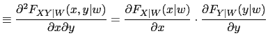
In general, if you know two marginal distributions, you cannot derive the joint distribution. However, when marginal distributions are continuous, a joint distribution can be recovered from the marginal distributions with the use of a copula. According to Sklar's (1959) theorem, the copula enables the construction of bivariate (multivariate) densities that are consistent with the univariate marginal densities. This allows for a separation of the specification of the dependence structure and the univariate marginal distributions.
Let ![]() be the joint distribution of
be the joint distribution of
![]() and
and ![]() ,
, ![]() the marginal distribution of
the marginal distribution of ![]() and
and
![]() the marginal distribution of
the marginal distribution of ![]() . Then
. Then
| (1) |
where ![]() indicates the copula, i.e. the dependence
structure that puts together the marginal information contained in
indicates the copula, i.e. the dependence
structure that puts together the marginal information contained in
![]() and
and ![]() . Similarly
. Similarly
| (2) |
where ![]() and
and ![]() represent the
marginal densities of
represent the
marginal densities of ![]() and
and ![]() ,
respectively,
,
respectively, ![]() is the second-order derivative of the
copula w.r.t. the marginals, and
is the second-order derivative of the
copula w.r.t. the marginals, and ![]() is the joint
density of
is the joint
density of ![]() and
and ![]()
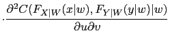
As derived in Patton (2006b), the conditional copula of
![]() can be obtained given just the
unconditional copula of
can be obtained given just the
unconditional copula of ![]() and the marginal
density of
and the marginal
density of ![]() , so that the conditional copula
becomes
, so that the conditional copula
becomes
| (3) |
However, in order for ![]() to be the joint
conditional distribution function and for Sklar's theorem to hold
for the conditional copula, the conditioning variables included in
to be the joint
conditional distribution function and for Sklar's theorem to hold
for the conditional copula, the conditioning variables included in
![]() must be the same for both marginal
distributions and the copula . The only exception is if a part of
must be the same for both marginal
distributions and the copula . The only exception is if a part of
![]() , say
, say ![]() ,
,![]() only affects the conditional
distribution of one variable but not the other.
only affects the conditional
distribution of one variable but not the other.
As shown in Patton (2006b) the density function to be used for
maximum likelihood estimation is easily obtained provided that
![]() and
and ![]() are differentiable and
are differentiable and ![]() and
and ![]() are twice differentiable:
are twice differentiable:
|
||
|
(4) | |
| (5) |
so
| (6) |
where
![]() and
and
![]() ,
,
![]()
![]()
![]() and
and
![]() .
This shows that we can evaluate each piece of the likelihood
separately. Estimates will be consistent, but could be inefficient.
However, given our very long data set this will not be an
issue.
.
This shows that we can evaluate each piece of the likelihood
separately. Estimates will be consistent, but could be inefficient.
However, given our very long data set this will not be an
issue.
Therefore, in our set up, what we need is a model for the
marginal distributions of the various exchange rate returns and a
functional form for the copula. Following most of the exchange rate
literature, we model exchange rate returns using a ![]() specification. It is important that the marginal
densities are well specified. The use of a mis-specified model for
the marginal distributions leads to probability integral transforms
which will not be
specification. It is important that the marginal
densities are well specified. The use of a mis-specified model for
the marginal distributions leads to probability integral transforms
which will not be
![]() , and so any copula model will
automatically be mis-specified. More details on this are provided
in Section 4.
, and so any copula model will
automatically be mis-specified. More details on this are provided
in Section 4.
In terms of choice of the copula functions, we use two specifications: the Normal copula and the symmetrized Joe-Clayton copula (SJC), both with constant and time-varying parameters. The Normal copula will give us the correlation, the traditional dependency measure, while the Joe-Clayton copula will give us the tail dependencies, which are the ones we are interested in here. Breymann, Dias and Embrechts (2003) show there exist clustering of extreme returns in the odd quadrants, so that positive (negative) returns for one currency tend to be associated with positive (negative) returns for the other currency. These are the two quadrants that the Joe-Clayton copula studies.
The Normal copula is
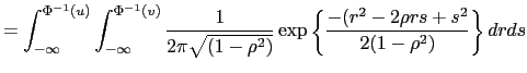
|
(7) | |
| (8) |
where ![]() is the inverse of the standard
normal c.d.f, while the symmetrized Joe-Clayton Copula is
is the inverse of the standard
normal c.d.f, while the symmetrized Joe-Clayton Copula is
![$\displaystyle C_{SJC}(u,v\vert\tau^{U},\tau^{L})=0.5\left( \begin{array}[c]{c} C_{JC}(u,v\vert\tau^{U},\tau^{L})\\ +C_{JC}(1-u,1-v\vert\tau^{L},\tau^{U})+u+v-1 \end{array} \right)$](img56.gif)
|
(9) |
where ![]() is Joe Clayton copula. The
is Joe Clayton copula. The ![]() is a weighted average of the Joe Clayton copula and
the survival Joe Clayton copula. The Joe Clayton copula is
is a weighted average of the Joe Clayton copula and
the survival Joe Clayton copula. The Joe Clayton copula is
| (10) | ||
| (11) | ||
| (12) | ||
| (13) |
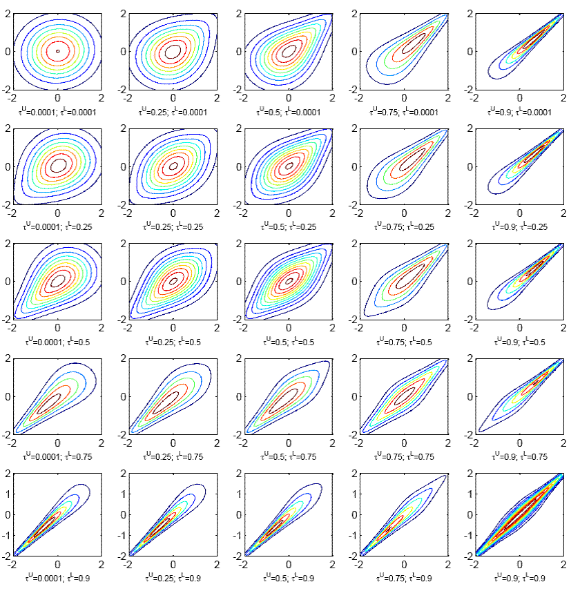
Parameters of interest in the study of exchange rates dependence
are the correlation ![]() in the normal copula,
and the upper tail dependence
in the normal copula,
and the upper tail dependence
![]() and the lower tail dependence
and the lower tail dependence
![]() in the symmetrized Joe-Clayton
copula. It is well known how the normal distribution varies with
in the symmetrized Joe-Clayton
copula. It is well known how the normal distribution varies with
![]() : with
: with ![]() the contours
of the distribution look very much like concentric circles, and as
the contours
of the distribution look very much like concentric circles, and as
![]() increases the contours stretch out along
the 45 degree line. The interpretation of
increases the contours stretch out along
the 45 degree line. The interpretation of ![]() and
and ![]() is a little bit trickier.
is a little bit trickier.
![]() and
and ![]() govern
the upper and the lower tails of the distribution, respectively.
When
govern
the upper and the lower tails of the distribution, respectively.
When
![]() , the distribution is
symmetric, as the panels on the main diagonal of Figure 1 show. When
, the distribution is
symmetric, as the panels on the main diagonal of Figure 1 show. When
![]() , the contours of the
distribution become thinner in the upper tail, meaning that if you
get a realization for
, the contours of the
distribution become thinner in the upper tail, meaning that if you
get a realization for ![]() (
(![]() ) in the upper
tail, the probability of getting a realization of
) in the upper
tail, the probability of getting a realization of ![]() (
(![]() ) in the upper tail is high. Similarly,
when
) in the upper tail is high. Similarly,
when
![]() , the contours of the
distribution become thinner in the lower tail, meaning a higher
probability of joint realization of
, the contours of the
distribution become thinner in the lower tail, meaning a higher
probability of joint realization of ![]() and
and
![]() in the lower tail. The off-diagonal panels
in Figure 1 illustrate these concepts. In our framework, when the difference
between the upper and lower tail parameters is zero, the bivariate
distribution is symmetric; when the difference between the upper
and lower tail parameters is negative, there is a greater
probability that the dollar will depreciate jointly versus two
foreign currencies. This can be seen as the contours get thinner in
the lower tail. Vice-versa, when the difference is positive,
there is a greater probability that the dollar will appreciate
jointly versus two foreign currencies.
in the lower tail. The off-diagonal panels
in Figure 1 illustrate these concepts. In our framework, when the difference
between the upper and lower tail parameters is zero, the bivariate
distribution is symmetric; when the difference between the upper
and lower tail parameters is negative, there is a greater
probability that the dollar will depreciate jointly versus two
foreign currencies. This can be seen as the contours get thinner in
the lower tail. Vice-versa, when the difference is positive,
there is a greater probability that the dollar will appreciate
jointly versus two foreign currencies.
The ![]() ,
, ![]() , and
, and
![]() parameters in Equations (8) and (13) are fixed across
time. However, they can be made time varying. Here we consider the
following evolution equations for the dependence parameters:
parameters in Equations (8) and (13) are fixed across
time. However, they can be made time varying. Here we consider the
following evolution equations for the dependence parameters:
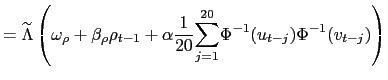
|
(14) | |
|
(15) | |
|
(16) | |
Equations (14) and
(16) imply that the
dependence parameters follow a kind of an ARMA(1,20) process. The
AR regressor is present to capture the persistence in the
dependence or the tail dependence of the parameter. We also include
a mean-reverting forcing variable in the tail dependence evolution
equations, and for compatibility the last term in the evolution
equation for the correlation will capture variations in the
dependence over the last twenty days. To keep ![]() within
within ![]() , and
, and ![]() and
and ![]() within the
within the
![]() bounds, the ARMA equations are
transformed with
bounds, the ARMA equations are
transformed with
![]() in the normal case and
in the normal case and
![]() in the symmetrized Joe-Clayton
case.2
in the symmetrized Joe-Clayton
case.2
3. Data
The data set is composed of daily returns of the six main bilateral exchange rates against the U.S. dollar: Australian dollar (AUD), Canadian dollar (CAD), Swiss franc (CHF), euro (EUR), British pound (GBP), and Japanese yen (YEN). It spans the period January 2, 1980 to November 15, 2007. All the exchange rates are quoted as foreign currency per USD so that if the exchange rate increases (decreases), the foreign currency is depreciating (appreciating) against the USD. We construct the euro returns series by concatenating Deutsche Mark (DM) returns before January 1, 1999 and euro returns from 1999 onward. We delete dates for which at least one of the markets was closed, and January 4, 1999, because there is no observation for the EUR return series due to the switch from DM to EUR. We also delete dates for which the absolute return of one of the series was greater than 5 percent: AUD returns are greater than 5 percent on three dates: March 3, 1983; February 19, 1985; and February 21, 1985. YEN returns are greater than 5 percent on October 7, 1998.3
Table 1 depicts the summary statistics for the returns series of the six bilateral exchange rates analyzed in the paper. Mean and median are always approximately zero, while the standard deviation ranges from 36 for the Canadian dollar to 76 for the Swiss franc. CHF , EUR and YEN exhibit negative skewness, AUD and CAD reveal positive skewness, and GBP displays small but positive skewness. All series exhibit excess kurtosis, and the Jarque-Bera test of normality of the unconditional distribution rejects unconditional normality for all series at the 1 percent level. Figure 2 displays the exchange rate returns series. The Canadian dollar is less volatile than the other series, especially in the first part of the sample.
Unconditional pairwise correlation coefficients, as shown in Table 2, range from 0.11 to 0.93. The lowest and highest correlations characterize the pairs Yen - Canadian dollar and Swiss franc - euro, respectively. A higher degree of unconditional linear correlation is exhibited between the European currencies than between the other currency pairs.
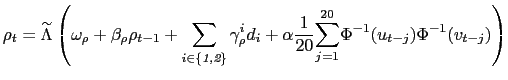
The data set also includes business cycle dummies, see Table 3, which are equal to 1 during expansions (from trough to peak) and zero otherwise.4 These dummies will be used to asses whether and how pairwise dependence between currency pairs is affected by business cycles.
In order to look at the effects of interest rate differentials on the dependence structures over time, we collect three-month Libor rates and ten-year sovereign bond yields. Based on data availability, the biggest common sample we use with interest rate data spans the period October 24, 1994 to November 15, 2007.
We use a dummy, equal to 1 from the beginning of 1999, for the Canadian and the Australian dollars. Although there is no major event, we observed an increased volatility of the returns, especially in Canada, in the second part of the sample, and we therefore try to correct for such a change by including a dummy in the marginal estimation. A dummy is also included to account for the switch from Deutsche mark to euro.
4. Models for the Marginal Distributions
We model the marginal distributions of the exchange rates using
a ![]() ,
,
![]() specification:
specification:
| (17) | ||
| (18) | ||
|
(19) |
where
![]() are the
exchange rate returns,
are the
exchange rate returns,
![]() are lagged returns,
and
are lagged returns,
and
![]() is the degrees of freedom
parameter.
is the degrees of freedom
parameter.
The model for the conditional copula requires the conditioning information set to be the same in both marginal models employed in the copula and in the copula itself, hence any variable that we want to include in the copula models has to be included in the marginals as well (unless these variables turn out to be not significant statistically in the marginals). Because of this, we have five sets of marginal models to be estimated:
(a) marginal distributions with no other explanatory variables other than lagged endogenous variables (" Plain" model),
(b) marginal distributions with lagged endogenous variables and foreign dummy recessions (" Foreign recession" model),
(c) marginal distributions with lagged endogenous variables and U.S. dummy recession (" US recession" model),
(d) marginal distributions with lagged endogenous variables and three-month interest rate data (" Three-month rates" model),
(e) marginal distributions with lagged endogenous variables and ten year interest rate data (" Ten-year rates" model).
Within each model, we actually have 15 marginal distributions to be estimated (all the possible currency pair combinations). Each marginal distribution for the same exchange rate might differ across models (a) through (e) due to the fact that different explanatory variables are used in each one of these models.
So for example, for model (a), the " plain" model, we start by
estimating marginal distributions where exchange rate returns are
regressed only on their own lagged values in the mean equation. We
choose the best specification according to SIC, AIC, residuals and
squared residuals tests. Table 4 reports
parameter estimates and standard errors for the best
specifications. The selected marginal models are:
![]()
![]() , with inclusion of the regime
dummy both in the mean and in the variance equations, for the
Australian dollar;
, with inclusion of the regime
dummy both in the mean and in the variance equations, for the
Australian dollar; ![]()
![]() , with dummy in mean and
variance equations, for the Canadian dollar;
, with dummy in mean and
variance equations, for the Canadian dollar; ![]()
![]() for the Swiss franc;
for the Swiss franc;
![]()
![]() , with dummy in the mean
equation, for the euro;
, with dummy in the mean
equation, for the euro; ![]()
![]() for sterling;
for sterling;
![]() for the Japanese
yen.5 However, as already pointed out, the
model for the conditional copula requires the conditioning
information set to be the same for both marginal models employed in
the copula. We need therefore under model (a) to test for the
significance of lags of other exchange rate returns both in the
mean and in the variance equations.6 Some other lagged
exchange rate returns turn out to be significant in the mean
equation, and therefore those need to be included in the model
specification to obtain the marginal distributions that we can use
to retrieve the copula. In contrast, no lags of other exchange rate
returns are significant in the variance equations. We therefore
update the marginal distribution with cross exchange rate lags.
for the Japanese
yen.5 However, as already pointed out, the
model for the conditional copula requires the conditioning
information set to be the same for both marginal models employed in
the copula. We need therefore under model (a) to test for the
significance of lags of other exchange rate returns both in the
mean and in the variance equations.6 Some other lagged
exchange rate returns turn out to be significant in the mean
equation, and therefore those need to be included in the model
specification to obtain the marginal distributions that we can use
to retrieve the copula. In contrast, no lags of other exchange rate
returns are significant in the variance equations. We therefore
update the marginal distribution with cross exchange rate lags.
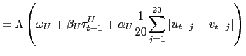
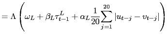
Similar steps are taken to estimate the marginal distributions for models (b)-(e). To conserve space we do not report these results. A few remarks, however, are in order. In model (b), when looking at currency pairs of the type foreign-currency-1/USD and foreign-currency-2/USD, we need to include recession cycles for both country 1 and country 2. That means, we include in the marginal regression for each exchange rate both its own country's recession dummy, and also country 2's recession dummy.7 In model (c), the U.S. dummy variables are not significant, and therefore the marginals are identical to the marginals in the plain model. Interest rate models (d) and (e) include three-month and ten-year interest rate differentials (country 1's rate minus country 2's rate) in the marginal distributions.8
4.1 Testing the Marginal Models
It is very important that the models for the marginal
distributions are indistinguishable from the true marginal
distributions. Mis-specified models for the marginal distributions
will result in mis-specified copula models. The probability
integral transforms of the residuals from the marginal models
![]() and
and
![]() , have to be
, have to be
![]()
We employ simple tests of
![]() such as the
Kolmogorov-Smirnov test and the Cramer-von Mises test. We also test
formally for the independence of the first four moments of the
transformed series by regressing
such as the
Kolmogorov-Smirnov test and the Cramer-von Mises test. We also test
formally for the independence of the first four moments of the
transformed series by regressing
![]() on 40 lags
of
on 40 lags
of
![]() where
where
![]() and
and ![]() AUD, CAD,
CHF, EUR, GBP and Yen. In addition, similar to what Diebold,
Gunther and Tay (1998) recommended, we use graphical methods to
supplement these more formal tests (see Appendix 2). Table 5 shows the test
for model (a), the " plain" model.9 The null hypothesis that
the marginal models are correctly specified can almost never be
rejected. The p-values for the LM test and the Kolmogorov-Smirnov
test are always equal to or greater than ten percent, while the
Cramer-von Mises test is rejected at the five percent level for the
yen. Since the LM test is not rejected for the yen we continue our
analysis without changing the marginal model further.
AUD, CAD,
CHF, EUR, GBP and Yen. In addition, similar to what Diebold,
Gunther and Tay (1998) recommended, we use graphical methods to
supplement these more formal tests (see Appendix 2). Table 5 shows the test
for model (a), the " plain" model.9 The null hypothesis that
the marginal models are correctly specified can almost never be
rejected. The p-values for the LM test and the Kolmogorov-Smirnov
test are always equal to or greater than ten percent, while the
Cramer-von Mises test is rejected at the five percent level for the
yen. Since the LM test is not rejected for the yen we continue our
analysis without changing the marginal model further.
We also tested formally for the independence of the first four
moments of the transformed series by regressing
![]() on 40 lags
of itself and one other currency
on 40 lags
of itself and one other currency
![]() where
where
![]() and
and
![]() and
and ![]() . This is a bivariate version of the LM test. For the
plain models, only 6 out of the 120 p-values are below the five
percent critical value, with no apparent pattern to which
currencies are involved.10
. This is a bivariate version of the LM test. For the
plain models, only 6 out of the 120 p-values are below the five
percent critical value, with no apparent pattern to which
currencies are involved.10
5. Models for the Copula
Maximum likelihood is used to estimate the bivariate normal copula models and the bivariate symmetrized Joe-Clayton models. This procedure, which separates the estimation of the marginals from the estimation of the copulas, was proposed by Patton (2006b) and is appropriate for large samples. For each copula model, 14 pairs are estimated.11 Under standard conditions the estimates obtained are consistent and asymptotically normal.
5.1 Exchange Rates Dependence - "Plain Models"
We start by estimating the copulas using probability integral transforms of the residuals from the "plain" models, which only included lagged endogenous explanatory variables. In line with the marginal models, the resulting copulas will be referred to as the plain normal copula and the plain SJC-copula.
Constant Copula Results
The estimates for the plain constant normal copula and the plain
constant SJC-copula (equations 7 and 9) are presented
in Table 6. As
would be expected, the estimates for ![]() in the
normal copula are very close to linear pairwise correlations in
Table 2.
in the
normal copula are very close to linear pairwise correlations in
Table 2.
We are, however, interested in knowing if estimating the tail
dependence gives us any additional information about the dependence
structure over and above the simple linear pairwise correlations.
In seven of the fourteen copulas, the difference between the upper
and lower tail dependence is significant, confirming that the
dependence structure is not symmetric. The SJC copula is therefore
picking up deviations from symmetry, which would be lost with the
use of either normal or Student's t distribution assumptions. With
no exogenous dependent variable ![]() is
significantly greater than
is
significantly greater than ![]() in five
instances, while it is significantly smaller only twice.
in five
instances, while it is significantly smaller only twice.
![]() greater than
greater than ![]() means that the pairs are more likely to experience
joint steep appreciation against the dollar, rather than joint
steep depreciation. If we turn that around, this result suggests
that the dollar takes the escalator down when it depreciates
against foreign currencies while it takes the stairs up when it
appreciates against foreign currencies. It is interesting to note
that exceptions to this occurs in pairs that include the Japanese
yen, where in two copulas
means that the pairs are more likely to experience
joint steep appreciation against the dollar, rather than joint
steep depreciation. If we turn that around, this result suggests
that the dollar takes the escalator down when it depreciates
against foreign currencies while it takes the stairs up when it
appreciates against foreign currencies. It is interesting to note
that exceptions to this occurs in pairs that include the Japanese
yen, where in two copulas ![]() is
significantly higher than
is
significantly higher than ![]() . Michelis
and Ning (2008), within a framework similar to ours, also find
asymmetric static and dynamic tail dependence between the Canadian
stock market and the US/Canada real exchange rate. This suggests
that asymmetric dependence is important non only in foreign
exchange markets, but also across markets.
. Michelis
and Ning (2008), within a framework similar to ours, also find
asymmetric static and dynamic tail dependence between the Canadian
stock market and the US/Canada real exchange rate. This suggests
that asymmetric dependence is important non only in foreign
exchange markets, but also across markets.
Time-Varying Copula Results
The results for the time-varying normal copulas (equation
14) are presented
in the first three columns of Table 7. The parameter
estimates are mostly significant at the five percent level. As can
be seen in the second column in Table 7,
![]() is always significantly
positive, meaning that the time-varying normal copulas exhibit a
positive autocorrelation for the correlation between all of the
currency pairs.
is always significantly
positive, meaning that the time-varying normal copulas exhibit a
positive autocorrelation for the correlation between all of the
currency pairs.
![]() , the third column, is positive
everywhere but once, meaning that high average variation in the
dependency between currency movements in the last twenty trading
days implies high correlation between them in the current period.
Figure 3 plots
the conditional correlation for the time-varying normal copula. It
is apparent that the euro and the Swiss franc move very closely
over the period analyzed, substantiating our decision to disregard
these pairs in our estimation. It may also be worth exploring why
the time-varying correlation between the Canadian dollar and the
other currencies, most notably euro and Swiss franc, seems to go
down in the early 90's and then slowly up again.
, the third column, is positive
everywhere but once, meaning that high average variation in the
dependency between currency movements in the last twenty trading
days implies high correlation between them in the current period.
Figure 3 plots
the conditional correlation for the time-varying normal copula. It
is apparent that the euro and the Swiss franc move very closely
over the period analyzed, substantiating our decision to disregard
these pairs in our estimation. It may also be worth exploring why
the time-varying correlation between the Canadian dollar and the
other currencies, most notably euro and Swiss franc, seems to go
down in the early 90's and then slowly up again.
Table 7 also
exhibits the results for the estimations of the time-varying SJC
copulas (equations 15 and 16). The tail
dependence exhibits negative autocorrelation, that is ![]() and
and ![]() are negative,
indicating that extreme co-movements do not happen in clusters. The
forcing parameters
are negative,
indicating that extreme co-movements do not happen in clusters. The
forcing parameters
![]() and
and
![]() are also negative. The
time-varying lower tail dependence and the upper tail dependence
are presented in Figures 4 and 5. The tail
dependence is varies greatly over time for the currency pairs. This
can be seen as the movements of the time-varying estimates are very
frequently well outside the 95 percent confidence interval around
the constant estimates of the dependency parameters.
are also negative. The
time-varying lower tail dependence and the upper tail dependence
are presented in Figures 4 and 5. The tail
dependence is varies greatly over time for the currency pairs. This
can be seen as the movements of the time-varying estimates are very
frequently well outside the 95 percent confidence interval around
the constant estimates of the dependency parameters.
5.2 Exchange Rates Dependence and Business Cycles
The outcome of the plain copula models affirms our hypothesis that fitting a symmetric bivariate distribution to exchange rate co-movements would, in most cases, not be sufficient. Moreover, it is also apparent that there is a lot of variation over time both in the correlation and in the tail parameters. Hence, we go a step further here and add exogenous variables to the models, first and foremost to see if these exogenous variables affect the time-varying dependence structures, but also to see if their inclusion changes the outcome of the constant copulas. First we would like to see if the business cycle influences the estimated dependence structures, and then we will look at the effects of interest rate differentials.
5.2.1 Business Cycles Results
We estimate the copulas using probability integral transforms of the residuals from i) foreign recession marginal models and ii) U.S. recessions marginal models.
Foreign Recessions
Constant Copula
The result for the constant foreign recession SJC-copulas are presented in the upper half of Table 8.12 There is a significant difference between the upper and lower tail dependence in seven out of the 14 copulas, so conditioning on the business cycle in the marginal models does not eliminate the asymmetry in the bivariate distributions. When conditioning on foreign recessions the lower tail is significantly higher than the upper tail in five SJC-copulas, which is very similar to the outcome in the constant plain SJC copulas. Exceptions to this include the pairs Japanese yen - Swiss franc and Japanese yen - euro. Yen and Swiss franc are currencies that are frequently mentioned as potential " carry trade" currencies.
Time-Varying Copula Results
The equations for the estimation of the time-varying copulas have to be modified slightly to include the exogenous variables we are including in the marginals. For the time-varying foreign recession normal copula, a term is added to include the dummies for recessions. The new time evolution equation becomes:
|
(20) |
where
![]()
![]() first country recession, second country
recession
first country recession, second country
recession![]() , and the dummy
, and the dummy ![]() is 0
during a recession and
is 0
during a recession and ![]() otherwise so that if
otherwise so that if
![]() the
correlation
the
correlation ![]() is higher (lower) during
recessions in country
is higher (lower) during
recessions in country ![]() .
.
The modified equations for the time-varying foreign recession
SJC copulas also include the new parameters,
![]() and
and
![]() , with the same interpretation
as the new term in the time-varying normal copula.
, with the same interpretation
as the new term in the time-varying normal copula.
The results of the estimation of the time-varying foreign
recession normal copula and the time-varying foreign recession SJC
copula are presented in the first six columns of Table 9 For
abbreviation, we only report outcomes for the exogenous recession
parameters, that is
![]() and
and
![]() for
for
![]() .13 For the time-varying
foreign recession normal copula (columns one and two) the country
recessions are often not significant: out of 28 parameter
estimations, only 7 are significant. However, there seems to be
some pattern to this, as a recession in Japan seems to lower the
correlation between currency pairs (that is
.13 For the time-varying
foreign recession normal copula (columns one and two) the country
recessions are often not significant: out of 28 parameter
estimations, only 7 are significant. However, there seems to be
some pattern to this, as a recession in Japan seems to lower the
correlation between currency pairs (that is
![]() ) and significantly
so in four out of five cases. More specifically, a recession in
Japan lowers the correlation between the yen and the Australian
dollar, the Swiss franc, the Euro, and sterling. Any other
significant parameter has the opposite effect (see bold numbers in
first column of Table 9), that is, a
recession in Australia increases the correlation between the
Australian dollar and Swiss franc, a recession in Canada increases
the correlation between the Canadian dollar and sterling, and a
recession in Switzerland increases the correlation between the
Swiss franc and sterling.
) and significantly
so in four out of five cases. More specifically, a recession in
Japan lowers the correlation between the yen and the Australian
dollar, the Swiss franc, the Euro, and sterling. Any other
significant parameter has the opposite effect (see bold numbers in
first column of Table 9), that is, a
recession in Australia increases the correlation between the
Australian dollar and Swiss franc, a recession in Canada increases
the correlation between the Canadian dollar and sterling, and a
recession in Switzerland increases the correlation between the
Swiss franc and sterling.
Similar patterns can be seen for the effect of foreign
recessions on the lower and upper tail dependence, although there
are a few exceptions here. In most cases, when significant, a
recession in a country increases the lower and upper tail
dependence between currency pairs (that is
![]() ), while notable
exceptions are recessions in Japan. During a recession in Japan,
upper and lower tail dependence between the yen and the Canadian
dollar, the yen and the Euro, and the yen Sterling decline; the
lower tail dependence also decreases between the yen and the
Australian dollar.
), while notable
exceptions are recessions in Japan. During a recession in Japan,
upper and lower tail dependence between the yen and the Canadian
dollar, the yen and the Euro, and the yen Sterling decline; the
lower tail dependence also decreases between the yen and the
Australian dollar.
U.S. Recessions
Constant Copula
For the constant U.S. recession SJC-copulas (lower half of Table 8) the results are the same as for the constant plain SJC copulas, as the U.S. recession was not significant in any of the marginals. Even though business cycles in the U.S. do not affect individual currency marginals, we are still very interested in exploring if they affect the time-varying dependence structure between the currencies.
Time-Varying Copula Results
The model definitions for the time-varying U.S. recession copula
models are similar to those for the foreign recession models. The
time evolution equation for the normal copula, equation (20), changes so
that
![]() US recession
US recession![]() . Similar changes are made to the time-varying SJC copula.
Only 7 out of 42 estimates are significant (see the last three
columns in Table 9) for the
correlation, the upper and lower tail dependence. A recession in
the U.S. increases the correlation between the Canadian dollar and
the Swiss franc, and also between the Swiss franc and Sterling.
These are the only two currency pairs where the U.S. business cycle
affects the time-varying Gaussian correlation. The U.S. business
cycle never affects the time-varying upper tail dependence between
currency pairs, while interestingly it increases the lower tail
dependence (
. Similar changes are made to the time-varying SJC copula.
Only 7 out of 42 estimates are significant (see the last three
columns in Table 9) for the
correlation, the upper and lower tail dependence. A recession in
the U.S. increases the correlation between the Canadian dollar and
the Swiss franc, and also between the Swiss franc and Sterling.
These are the only two currency pairs where the U.S. business cycle
affects the time-varying Gaussian correlation. The U.S. business
cycle never affects the time-varying upper tail dependence between
currency pairs, while interestingly it increases the lower tail
dependence (
![]() significant at the 5
percent level) for 5 out of 14 currency pairs (AUD/GBP, CAD/GBP,
EUR/GBP, EUR/YEN and GBP/YEN).14 This means that if there is a
recession in the US, these currencies are more likely to experience
a joint steep appreciation against the dollar, than during other
periods. This would mean that the dollar takes an even faster
escalator down when there is a recession in the U.S. than during
other periods.
significant at the 5
percent level) for 5 out of 14 currency pairs (AUD/GBP, CAD/GBP,
EUR/GBP, EUR/YEN and GBP/YEN).14 This means that if there is a
recession in the US, these currencies are more likely to experience
a joint steep appreciation against the dollar, than during other
periods. This would mean that the dollar takes an even faster
escalator down when there is a recession in the U.S. than during
other periods.
This result does indicate that the time-varying Gaussian correlation between currency pairs is rarely affected by U.S. recessions. On the contrary, there seems to be some evidence that the U.S. recession affects the lower tail of the bivariate distribution. This means that just looking at the time-varying Gaussian correlation would potentially be misleading.
5.3 Exchange Rates Dependence and Interest Rate Differentials
It is widely recognized that interest rate differentials are not good predictors of nominal exchange rate movement. This point was established first by Meese and Rogoff in a seminal paper in 1983 and has since been emphasized by numerous other papers. Some papers can find some predictability for nominal exchange rate movement over a long horizon, such as Mark (1995), who, however, did not use interest rate differentials as one of the explanatory variables. Cheung et. al. (2005) even find that different structural models perform differently for different currencies, but they do declare the interest rate parity model as the winner for long horizon dollar-yen exchange rate predictions. Given this literature, we were interested in exploring whether interest rate differentials affect even the short run changes in the dependence structure between currency pairs. We estimate the copulas using probability integral transforms of the residuals from i) three-month rate marginal models and ii) ten-year rate marginal models. Many of the results presented above change when interest rate differentials are used as dependent variables in the marginals and in the time varying copulas.
5.3.1 Three-month Interest Rates
Constant Copula
For the constant three-month rate SJC copulas, there is a significant difference between the upper and lower tail dependence in only 4 out of the 14 copulas, as apposed to 7 or 8 before, see Table 10. This does indicate that interest rate differentials explain some of the asymmetry we have observed in the constant dependence structures above.
Time-Varying Copula Results
How interest rate differentials affect the evolution of the
dependence between the currencies is of more interest to us. The
model definitions for the time-varying three-month rate copulas are
similar to those for the foreign recession model; see equation
(20). We will
now have
![]() absolute difference between
three-month rates
absolute difference between
three-month rates![]() , and we will estimate the
parameters,
, and we will estimate the
parameters,
![]() and
and
![]() .
.
The results for the time-varying three-month rate normal copula
and the time-varying three-month rate SJC copula are presented in
the first three columns of Table 11. The absolute
difference in the three-month Libor rates between the countries has
a significant effect on the correlation between the exchange rate
movements in 9 out of 14 of the normal copulas; see column one. Six
of these are negative (
![]() ), indicating that
the higher the interest rate differential between the countries,
the less these currencies tend to co-move. All three exceptions to
this include the Australian dollar. For the upper and lower tail
dependence, 10 out of the 24 estimates are significant (column 2
and 3). Of these ten, eight are negative (
), indicating that
the higher the interest rate differential between the countries,
the less these currencies tend to co-move. All three exceptions to
this include the Australian dollar. For the upper and lower tail
dependence, 10 out of the 24 estimates are significant (column 2
and 3). Of these ten, eight are negative (
![]() or
or
![]() ), implying that higher
interest rate differentials decreases the tail dependency between
the currency pairs. Again the exceptions to this include the
Australian dollar.
), implying that higher
interest rate differentials decreases the tail dependency between
the currency pairs. Again the exceptions to this include the
Australian dollar.
5.3.2 Ten-year Interest Rates
Constant Copula
The results for the ten-year rates and the three-month rates are very similar for the constant copulas: there is a significant difference between the upper and the lower tail in only 4 out of the 14 constant SJC copulas. These are exactly the currency pairs for which we get a significant difference between upper and lower tails in the three-month rate model, that is CHF-CAD, EUR-CAD, GBP-EUR and YEN-CHF.
Time-Varying Copula Results
The model definitions for the time-varying ten-year rate copulas
are similar to those for the three-month rate model above. We will
now have
![]() absolute difference between
ten-year rates
absolute difference between
ten-year rates![]() and we will estimate the parameters,
and we will estimate the parameters,
![]() . The
outcome of the estimation is in columns four through six in Table
11. The
absolute difference in the 10-year bond yields between the
countries has a significant effect on the correlation, as well as
on upper and lower tail dependence between the exchange rate
movements in 16 out of 42 cases. All of these estimates are
negative, that is
. The
outcome of the estimation is in columns four through six in Table
11. The
absolute difference in the 10-year bond yields between the
countries has a significant effect on the correlation, as well as
on upper and lower tail dependence between the exchange rate
movements in 16 out of 42 cases. All of these estimates are
negative, that is
![]() ,
,
![]() ,
,![]() and
and
![]() This means that
currencies that have a higher difference in long term interest
rates tend to move less closely together, not only on average but
also when extreme events occur.
This means that
currencies that have a higher difference in long term interest
rates tend to move less closely together, not only on average but
also when extreme events occur.
When the interest rate differentials affect the tail dependence, they also affect the correlation in the same direction (see the AUD/YEN pair and the CAD/CHF pair). However, this does not eliminate the importance of looking separately at the lower and upper tail dependence, as the upper tail dependence is much more frequently significantly affected by the interest rate differentials than the lower tail (7 vs. 2 times). This means that as the long term interest rate differentials increase there is a lower probability of joint extreme depreciations against the U.S. dollar. Knowing about these kind of asymmetries can be especially important for any kind of risk analysis, where extreme co-movements are more important than small normal day-to-day co-fluctuations in the exchange rates.
6. Conclusions
In this paper, we studied the dependence structure of exchange rate pairs in the form of correlation and tail dependence. The correlation gives information about how two currencies move together " on average" across the distribution. However, the correlation imposes symmetry in the way exchange rates co-move in the two tails of the distribution. With the view that this might be too big of a restriction when analyzing exchange rates, and following Patton (2006b), we studied the dependence/co-movement between exchange rate pairs also in the form of upper and lower tail dependence. Moreover, we analyzed the evolution of the correlation, upper and lower tail dependence parameters over time, and investigated whether these parameters are affected by business cycles and interest rate differentials.
Our results show that:
(i) In the constant copula models, the difference between the upper and the lower tail parameters tends to be negative (when significant) in the plain model and in the models with recessions, except when the yen is involved. A negative difference between the upper and the lower tail parameters means that the U.S. dollar is more likely to depreciate than appreciate jointly against the other currencies.
(ii) In the time-varying models, the dependence parameters fluctuate heavily over time and are well outside the 95 percent confidence bands of the constant estimates.
(iii) In the foreign recession model, in many cases when significant, a recession in a country tends to increase the dependence (correlation, upper and lower tail) between currency pairs. Notable exceptions are Japanese recessions, which tend to de-couple the yen from the other currencies.
(iv) The U.S. business cycle never affects the time variation in the upper tail dependence between currency pairs, but it increases the lower tail dependence for 5 out of 14 currency pairs, meaning that if there is a recession in the United States, some currencies are more likely to experience a joint steep appreciation against the dollar than during other periods.
(v) When significant, the effects of a higher interest rate differential are almost always negative, meaning that currencies with higher interest rate differentials tend to move less closely together, not only on average (correlation), but also when extreme events occur (tails). In the ten-year rate models, the upper tail dependence is much more frequently affected significantly by the interest rate differentials than the lower tail.
7. Appendix 1: Tail Dependence
If the limit
![$\displaystyle \underset{\varepsilon\rightarrow0}{\lim}\Pr[U\leq\varepsilon\vert V\leq \varepsilon]=\underset{\varepsilon\rightarrow0}{\lim}\Pr[V\leq\varepsilon \vert U\leq\varepsilon]=\underset{\varepsilon\rightarrow0}{\lim}\frac {C(\varepsilon,\varepsilon)}{\varepsilon}=\tau^{L} $](img193.gif)
![$\displaystyle \underset{\delta\rightarrow1}{\lim}\Pr[U>\delta\vert V>\delta]=\underset {\delta\rightarrow1}{\lim}\Pr[V>\delta\vert U>\delta]=\underset{\delta\rightarrow 1}{\lim}\frac{(1-2\delta+C(\delta,\delta))}{(1-\delta)}=\tau^{U} $](img197.gif)
8. Appendix 2: Testing Marginal Distributions
Here we present graphical methods to test if the probability
integral transforms are
![]() and i.i.d. Diebold, Gunther and
Tay (1998) argue that if the more formal tests applied above are
rejected, then it is hard to know what prompted the rejection, a
violation of i.i.d. or of unconditional uniformity. For
unconditional uniformity we will look at simple histograms of the
integral transforms,
and i.i.d. Diebold, Gunther and
Tay (1998) argue that if the more formal tests applied above are
rejected, then it is hard to know what prompted the rejection, a
violation of i.i.d. or of unconditional uniformity. For
unconditional uniformity we will look at simple histograms of the
integral transforms, ![]() . While sample
autocorrelation figures will be used to evaluate the i.i.d.
hypothesis. We look at the dependence structure in the conditional
mean
. While sample
autocorrelation figures will be used to evaluate the i.i.d.
hypothesis. We look at the dependence structure in the conditional
mean
![]() , conditional variance
, conditional variance
![]() , conditional skewness
, conditional skewness
![]() , and conditional
kurtosis
, and conditional
kurtosis
![]() . In 6-8 we see that the
histogram for the euro is slightly non-uniform in the range from
0.6 to 0.7, and the Swiss franc and the Australian dollar both have
one bin noticeably outside the confidence interval. Apart from this
the distributions do not seem noticeably non-uniform. The
correlograms do not seem to find major flaws in the marginal
models; we have slight problems in the variance and the kurtosis,
most notably in the euro and the Canadian dollar.
. In 6-8 we see that the
histogram for the euro is slightly non-uniform in the range from
0.6 to 0.7, and the Swiss franc and the Australian dollar both have
one bin noticeably outside the confidence interval. Apart from this
the distributions do not seem noticeably non-uniform. The
correlograms do not seem to find major flaws in the marginal
models; we have slight problems in the variance and the kurtosis,
most notably in the euro and the Canadian dollar.
Finally we also test formally for the independence of the first
four moments of the transformed series by regressing
![]() on 40 lags
of itself and one other currency
on 40 lags
of itself and one other currency
![]() where
where
![]() and
and
![]() and
and ![]() . This is a bivariate version of the LM test in section
4.1. Table 22 presents the p values for the LM test of the
hypothesis that the marginal models are correctly specified. The
test rejects the null for the conditional variance of the sterling,
with respect to its own lags and the lags of the conditional
variance of the euro. The test also rejects the null for the
conditional kurtosis of the Australian dollar regressed on its own
lags and the lags of the euro, sterling and yen. The other 56
p-values are above the 5% critical value.
. This is a bivariate version of the LM test in section
4.1. Table 22 presents the p values for the LM test of the
hypothesis that the marginal models are correctly specified. The
test rejects the null for the conditional variance of the sterling,
with respect to its own lags and the lags of the conditional
variance of the euro. The test also rejects the null for the
conditional kurtosis of the Australian dollar regressed on its own
lags and the lags of the euro, sterling and yen. The other 56
p-values are above the 5% critical value.
References
Bouye, E., Gaussel, N., and Salmon, M. (2001) "Investigating Dynamic Dependence Using Copulae," mimeo.
Breymann, W., Dias, A. and Embrechts, P. (2003) " Dependence structures for multivariate high-frequency data in finance," Quantitative Finance 3(1), 1-16.
Cheung, Y.W., Chinn M.D. and Pascual A.G. (2005) " Empirical exchange rate models of the nineties: Are any fit to survive?" Journal of International Money and Finance, 24(7), 1150-1175.
Chollete, L., de la Pena, V., and Lu, C. (2008) " The Scope of International Diversification: Implications of Alternative Measures," mimeo.
Dias, A. and Embrechts, P. (2004) " Dynamic copula models for multivariate high-frequency data in finance," mimeo.
Diebold, Gunther and Tay (1998) " Evaluating Density Forecasts with Applications to Financial Risk Management," International Economic Review, 39, 863-883.
Embrechts, P., A. Mcneil and Straumann D., " Correlation and dependence in risk management," Properties and Pitfalls in Risk Management: Value at Risk and Beyond, ed. M.A.H. Dempster, (Cambridge University Press, Cambridge, 2002), 176-223.
Hurd, M, Salmon, M. and Schleicher, C. (2005) " Using Copulas to Construct Bivariate Foreign Exchange Distributions with an Application to the Sterling Exchange Rate," mimeo.
Jondeau, E. and Rockinger, M. (2006) " The Copula-GARCH model of conditional dependencies: An international stock market application," Journal of International Money and Finance, 25, 827-853.
Judd, K. L. (1998) Numerical Methods in Economics, MIT Press, Cambridge, Massachusetts.
Mark, N. (1995) " Exchange Rates and Fundamentals: Evidence on Long-Horizon Predictability," The American Economic Review, 85(1) 201-218.
Meese, R. and Rogoff, K. (1983) " Empirical exchange rate models of the seventies: Do they fit out of sample?" Journal of International Economics, 14(February) 3-24.
Michelis, L. and Ning, C. (2008) " The Dependence Structure between the Canadian Stock Market and the US/Canada Exchange Rate: A Copula Approach," mimeo.
Okimoto, T. (2008) " New Evidence of Asymmetric Dependence Structures in International Equity Markets," Journal of Financial and Quantitative Analysis, 43(3), 787-816.
Nelson, R.B., An introduction to copulas, Springer, New York, 1999.
Patton, A. (2006) " Estimation of Multivariate Models for Time Series of Possibly Different Lengths," Journal of Applied Econometrics, 21(2), 147-173.
Patton, A. (2006) " Modeling Asymmetric Exchange Rate Dependence," International Economic Review, 47(2), 527-556.
Rank, J. (2007) " Copulas: From theory to Aplication in Finance," London : Risk Books.
Salmon, M. and Bouye, E. (2008) " Dynamic Copula Quantile Regressions and Tail Area Dynamic Dependence in Forex Markets," mimeo.
Salmon, M. and Schleicher, C. (2006) " Pricing Multivariate Currency Options with Copulas," in Copulas, from theory to application in Finance, edited by Dr Jörn Rank RISK books.
Zimmer, D.M. and Trivedi, P.K. (2006) " Using Trivariate Copulas to Model Sample Selection and Treatment Effects: Application to Family Health Care Demand," American Statistical Association, 24, 63-76.
Figure 1. Symmetrized Joe-Clayton Copula
The 25 panels show how the contours of the symmetrized Joe-Clayton copula change with tau.
Figure 2. Exchange Rate Returns
![In Figure 2, a 2x3 grid of panels showing exchange rate returns for the six bilateral exchange rates analyzed in the paper (Australian dollar, Canadian dollar, Swiss franc, euro, British pound, and Japanese yen). All returns are presented as foreign currency against the U.S. dollar. The sample period for all returns is January 2, 1980 to November 15, 2007 (plotted on the x-axis) and the y-axis shows the daily return in the range [-4, 4]. Standard deviations of the daily returns range from 36 for the Canadian dollar to 76 for the Swiss franc.](Figure2.gif)
Exchange rate returns for the six bilateral exchange rates analized in the paper. All rates are against the U.S. dollar. The sample period is January 2, 1980 to Novemberr 15, 2007.
Figure 3. Time path of the correlation for the normal copula.
![In Figure 3, a 5x3 grid of panels showing the time path of the correlation for the normal copula for currency pairs. The y-axis time interval is over the period January 2, 1980 to November 15, 2007. The x-axis for each panel is the interval [-1, 1]. The euro and Swiss franc have a relative lack in time-variance, maintaining a near perfect correlation over the period studied. The time-varying correlation between the Canadian dollar and other currencies seems to fall in the early-1990s and then slowly rise in the latter part of the decade. For example, the correlation between the Canadian dollar and the Swiss franc is 02.-0.4 from the late 1980s to the period 1992-1993 and then falls significantly until reaching -0.3 levels in 1995. It then gradually increases up to its previous levels of 0.2 to 0.3 in 2002 and beyond.](Figure3.gif)
Figure 4. Time path of the time-varying lower tail dependence in the symmetrised Joe-Clayton copula
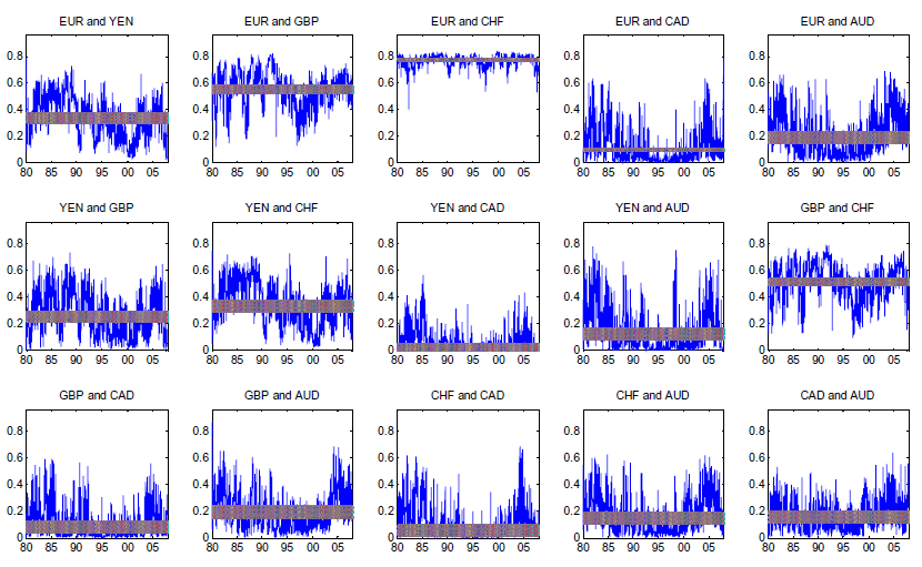
Figure 5. Time path of the time-varying upper tail dependence in the symmetrised Joe-Clayton copula
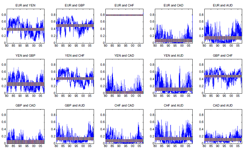
Figure 6. Statistics for The Euro-Yen Currency Pair

The two upper
panels are histograms of ![]() with 20 bins, with a 90
confidence interval under the null hypothesis of
with 20 bins, with a 90
confidence interval under the null hypothesis of
![]() ). The bottom panels are the
sample autocorrelations for the conditional mean (1), conditional variance (2), conditional skewness (3), and conditional kurtosis(4).
). The bottom panels are the
sample autocorrelations for the conditional mean (1), conditional variance (2), conditional skewness (3), and conditional kurtosis(4).
Figure 7. Statistics for The Pound-Swiss Franc Currency Pair
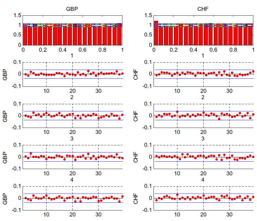
The two upper
panels are histograms of ![]() with 20 bins, with a 90
confidence interval under the null hypothesis of
with 20 bins, with a 90
confidence interval under the null hypothesis of
![]() . The bottom panels are the
sample autocorrelations for the conditional mean (1), conditional
variance (2), conditional skewness (3), and conditional kurtosis
(4).
. The bottom panels are the
sample autocorrelations for the conditional mean (1), conditional
variance (2), conditional skewness (3), and conditional kurtosis
(4).
Figure 8. Statistics for The Canadian-Australian Dollar Currency Pair
The two upper
panels are histograms of ![]() with 20 bins, with a 90%
confidence interval under the null hypothesis of
with 20 bins, with a 90%
confidence interval under the null hypothesis of
![]() . The bottom panels are the
sample autocorrelations for the conditional mean (1), conditional
variance (2), conditional skewness (3), and conditional kurtosis
(4).
. The bottom panels are the
sample autocorrelations for the conditional mean (1), conditional
variance (2), conditional skewness (3), and conditional kurtosis
(4).
Table 1. Summary Statistics
| AUD | CAD | CHF | EUR | GBP | YEN | |
|---|---|---|---|---|---|---|
| Mean | 0.15 | -0.27 | -0.37 | -0.28 | 0.15 | -0.95 |
| Median | -1.74 | 0.00 | 1.66 | 1.22 | 0.00 | 0.68 |
| Std. Dev. | 63.81 | 36.12 | 75.86 | 69.11 | 64.58 | 70.28 |
| Skewness | 0.57 | 0.18 | -0.19 | -0.13 | 0.08 | -0.41 |
| Kurtosis | 7.50 | 6.97 | 4.57 | 5.32 | 6.58 | 6.35 |
| Jarque-Bera | 5644.36 | 4168.94 | 681.97 | 1435.15 | 3370.82 | 3127.21 |
| Nobs | 6301 | 6301 | 6301 | 6301 | 6301 | 6301 |
Note: The table shows summary statistics of the daily returns of AUD, CAD, CHF, EUR, GBP, and YEN expressed in basis points. The EUR series is constructed by concatenating DM returns and EUR returns. The sample period runs from January 2, 1980 to November 15, 2007, yielding 6301 observations. The asterisk (*) indicates rejection of the null hypotesys at the 0.01 percent level.
Table 2. Linear Pairwise Correlations
| AUD | CAD | CHF | EUR | GBP | YEN | |
|---|---|---|---|---|---|---|
| AUD | 1 | |||||
| CAD | 0.33 | 1 | ||||
| CHF | 0.25 | 0.21 | 1 | |||
| EUR | 0.28 | 0.22 | 0.93 | 1 | ||
| GBP | 0.29 | 0.22 | 0.70 | 0.73 | 1 | |
| YEN | 0.20 | 0.11 | 0.56 | 0.54 | 0.43 | 1 |
The table exhibits pairwise unconditional linear correlation for all the currency pairs analyzed in the paper. The highest degree of correlation is displayed between the European currencies, while the lowest correlation characterizes the CAD-CHF pair.
Table 3. International Business Cycle Dates
| 1979-1980: Peak | 1979-1980: Trough | 1981-1983: Peak | 1981-1983: Trough | 1984-1986: Peak | 1984-1986: Trough | 1987-1991: Peak | 1987-1991: Trough | 1992-1994: Peak | 1992-1994: Trough | 1995-1996: Peak | 1995-1996: Trough | 1997-1999: Peak | 1997-1999: Trough | 2000-2003: Peak | 2000-2003: Trough | 2004-2007: Peak | 2004-2007: Trough | |
|---|---|---|---|---|---|---|---|---|---|---|---|---|---|---|---|---|---|---|
| Australia | 6/82 | 5/83 | 6/90 | 12/91 | ||||||||||||||
| Canada | 4/81 | 11/82 | 3/90 | 3/92 | ||||||||||||||
| Switzerland | 9/81 | 11/82 | 3/90 | 9/93 | 12/94 | 9/96 | 3/01 | 3/03 | ||||||||||
| Euro Area | 1/80 | 10/82 | 1/91 | 4/94 | 1/01 | 8/03 | ||||||||||||
| United Kingdom | 5/81 | 5/90 | 3/92 | |||||||||||||||
| Japan | 4/92 | 2/94 | 3/97 | 7/99 | 8/00 | 4/03 | ||||||||||||
| United States | 1/80 | 7/80 | 7/81 | 11/82 | 7/90 | 3/91 | 3/01 | 11/01 |
The table displays business cycle dates for all the six countries considered in the paper, and for the United States, given that all bilateral exchange rates that we analyze are against the U.S. dollar. Data are not available for the period 2004-2007.
Table 4. Results for the Marginal Distributions - Panel A. Conditional Mean
| AUD | CAD | CHF | EUR | GBP | YEN | |
|---|---|---|---|---|---|---|
| Constant | | | | | | |
| Dummy | | | | |||
| AR(1) | | | | | ||
| AR(2) | | |||||
| AR(3) | | |||||
| AR(4) | | | | | ||
| AR(9) | | |||||
| AR(11) | | |||||
| Degrees of freedom | | | | | | |
The table reports maximum likelihood estimates for the AR t-Garch models of the marginal distributions. Only autoregressive lags that were selected in at least one specification are reported. Standard errors are in parenthesis. AR(m) refers to the autoregressive lag of the dependent variable; dummy indicates each country's own dummy.
Table 4. Results for the Marginal Distributions - Panel B. Conditional Variance
| AUD | CAD | CHF | EUR | GBP | YEN | |
|---|---|---|---|---|---|---|
| Constant | | | | | | |
| Resid(-1)^2 | | | | | | |
| Resid(-2)^2 | | | ||||
| Variance(-1) | | | | | | |
| Dummy | | | ||||
| Degrees of freedom | | | | | | |
The table reports maximum likelihood estimates for the AR t-Garch models of the marginal distributions. Only autoregressive lags that were selected in at least one specification are reported. Standard errors are in parenthesis. AR(m) refers to the autoregressive lag of the dependent variable; dummy indicates each country's own dummy.
Table 5. Testing of the Marginal Distribution Models
| AUD | CAD | CHF | EUR | GBP | YEN | |
|---|---|---|---|---|---|---|
| First moment LM test | 0.382 | 0.422 | 0.692 | 0.266 | 0.861 | 0.704 |
| Second moment LM test | 0.171 | 0.379 | 0.663 | 0.569 | 0.122 | 0.158 |
| Third moment LM test | 0.119 | 0.614 | 0.765 | 0.134 | 0.972 | 0.554 |
| Forth moment LM test | 0.303 | 0.544 | 0.348 | 0.600 | 0.195 | 0.156 |
| K-S test | 0.258 | 0.589 | 0.844 | 0.468 | 0.734 | 0.100 |
| Cramer-von Mises | 0.100 | 0.411 | 0.756 | 0.086 | 0.481 | 0.034 |
The table reports p-values from LM
tests of serial independence of the first four moments of the
probabilitiy integral transforms of the residual terms of the
marginal model. More specificly, for each probability
transforamtion of the residual term from the marginal model for
currencies (![]() where i=AUD, CAD, CHF, EUR, GBP
and YEN), the test is preformed by regressing
where i=AUD, CAD, CHF, EUR, GBP
and YEN), the test is preformed by regressing
![]() for n=1,2,3,4 onto
forty lags of
for n=1,2,3,4 onto
forty lags of ![]() i. For a p value less than 0.05
the null hypotheses that the marginal model is well-specified is
rejected. Here we also report the p-value for Kolmogorov-Smirnov
(KS) tests and the Cramer-vonMises tests for the uniform
distribution of the probability integral transforms of the residual
terms.
i. For a p value less than 0.05
the null hypotheses that the marginal model is well-specified is
rejected. Here we also report the p-value for Kolmogorov-Smirnov
(KS) tests and the Cramer-vonMises tests for the uniform
distribution of the probability integral transforms of the residual
terms.
Table 6. Constant Normal Copula
(![]() ) and Constant SJC copula (
) and Constant SJC copula (
![]() 391)- Plain
391)- Plain
| AUD | CAD | CHF | EUR | GBP | |
|---|---|---|---|---|---|
| CAD: | 0.3080 | ||||
| CAD: | 0.1152 | ||||
| CAD: | 0.1566 | ||||
| CAD: | -0.0414 | ||||
| CHF: | 0.3079 | 0.2152 | |||
| CHF: | 0.1404 | 0.0801 | |||
| CHF: | 0.1537 | 0.0600 | |||
| CHF: | -0.0133 | 0.0201 | |||
| EUR: | 0.3345 | 0.2311 | |||
| EUR: | 0.1527 | 0.0816 | |||
| EUR: | 0.1906 | 0.100 | |||
| EUR: | -0.0379 | -0.0184 | |||
| GBP: | 0.3417 | 0.2228 | 0.6861 | 0.7107 | |
| GBP: | 0.1419 | 0.0542 | 0.4869 | 0.503 | |
| GBP: | 0.194 | 0.0839 | 0.5150 | 0.5561 | |
| GBP: | -0.0521 | -0.0297 | -0.0281 | -0.0531 | |
| YEN: | 0.2683 | 0.1420 | 0.5725 | 0.5578 | 0.4372 |
| YEN: | 0.1199 | 0.0247 | 0.4218 | 0.3976 | 0.2633 |
| YEN: | 0.1271 | 0.0256 | 0.3358 | 0.3388 | 0.2539 |
| YEN: | -0.0072 | -0.0009 | 0.0860 | 0.0588 | 0.0094 |
The table shows the maximum likelihood estimates of the parameters of the constant normal and constant symmetrised-Joe-Clayton copula. All the estimates are highly significant at the 5 percent level. The italic numbers are the upper tail dependence minus the lower tail dependence, and they are bold if the difference is significant at the 10 percent level.
Table 7. Time-varying normal copula and SJC copula - Plain
| | | | | | | | |||
|---|---|---|---|---|---|---|---|---|---|
| AUD/CAD | 0.014 (0.007) | 0.111 (0.023) | 1.938 (0.043) | 2.835 (0.737) | -17.509 (2.729) | -3.265 (1.340) | 4.215 (0.592) | -21.039 (2.263) | -3.405 (0.671) |
| AUD/CHF | 0.055 (0.031) | 0.425 (0.131) | 1.527 (0.226) | 4.982 (0.555) | -26.266 (2.426) | -3.063 (0.616) | 4.336 (0.505) | -22.461 (2.143) | -3.309 (0.546) |
| AUD/EUR | 0.086 (0.037) | 0.568 (0.144) | 1.338 (0.246) | 4.612 (0.546) | -24.529 (2.476) | -3.004 (0.524) | 4.617 (0.399) | -22.501 (1.761) | -3.260 (0.382) |
| AUD/GBP | 0.158 (0.077) | 0.518 (0.178) | 1.146 (0.396) | 2.602 (0.849) | -17.478 (3.187) | -1.215 (1.039) | 3.587 (0.965) | -18.927 (3.298) | -2.074 (1.073) |
| AUD/YEN | 0.082 (0.043) | 0.707 (0.239) | 1.107 (0.396) | 4.470 (0.647) | -24.627 (2.630) | -2.260 (0.605) | 5.550 (0.406) | -28.999 (2.269) | -3.917 (0.216) |
| CAD/CHF | 0.002 (0.001) | 0.070 (0.011) | 2.000 (0.012) | 4.507 (0.749) | -25.334 (3.547) | -3.843 (0.716) | 4.930 (1.041) | -28.199 (4.336) | -2.220 (1.090) |
| CAD/EUR | 0.004 (0.002) | 0.086 (0.016) | 1.988 (0.019) | 4.366 (0.615) | -23.996 (2.746) | -3.682 (0.732) | 5.366 (0.832) | -28.730 (3.482) | -3.256 (0.886) |
| CAD/GBP | 0.419 (0.084) | 1.378 (0.211) | -1.240 (0.504) | 4.039 (0.957) | -24.726 (3.413) | -4.091 (1.356) | 5.232 (0.705) | -27.666 (2.396) | -2.956 (0.840) |
| CAD/YEN | 0.003 (0.002) | 0.068 (0.015) | 1.961 (0.021) | 6.844 (0.968) | -37.286 (4.609) | -4.469 (0.249) | 4.542 (1.228) | -28.455 (5.278) | -2.857 (1.373) |
| CHF/GBP | -0.088 (0.012) | 0.326 (0.021) | 2.307 (0.036) | 1.812 (0.008) | -10.290 (0.091) | -0.304 (0.014) | 1.752 (0.026) | -10.202 (0.040) | -0.005 (0.020) |
| CHF/YEN | 0.046 (0.015) | 0.410 (0.044) | 1.864 (0.060) | -0.464 (0.289) | -4.417 (0.918) | 2.438 (0.300) | 2.241 (0.153) | -13.727 (1.229) | -0.680 (0.261) |
| EUR/GBP | 0.075 (0.029) | 0.502 (0.043) | 1.951 (0.074) | 1.124 (0.000) | -8.511 (0.002) | 0.515 (0.000) | 1.294 (0.000) | -8.840 (0.000) | 0.614 (0.000) |
| EUR/YEN | 0.127 (0.041) | 0.601 (0.075) | 1.528 (0.135) | 1.263 (0.332) | -9.564 (0.978) | 0.653 (0.383) | 1.523 (0.748) | -11.206 (2.370) | -0.016 (0.906) |
| GBP/YEN | 0.232 (0.095) | 0.857 (0.175) | 0.855 (0.376) | 2.913 (0.715) | -16.251 (2.525) | -1.364 (0.827) | 4.406 (0.437) | -20.824 (2.030) | -3.477 (0.382) |
The table shows the maximum likelihood estimates of the parameters of the time-varying normal and time-varying symmetrised-Joe-Clayton copula. The numbers in the paranthesis are the asymptotic standard errors. Bold numbers indicate values for which we cannot reject the null hypothesis of a zero coefficient at the 5 percent level.
Table 8. Constant SJC copula - Foreign countries recessions and U.S. recessions - Panel A. Foreign Recession Copulas
| AUD | CAD | CHF | EUR | GBP | |
|---|---|---|---|---|---|
| CAD: | 0.1141 | ||||
| CAD: | 0.1586 | ||||
| CAD: | -0.0445 | ||||
| CHF: | 0.1395 | 0.0794 | |||
| CHF: | 0.1559 | 0.0608 | |||
| CHF: | -0.0164 | 0.0186 | |||
| EUR: | 0.1527 | 0.0914 | |||
| EUR: | 0.1912 | 0.0761 | |||
| EUR: | -0.0385 | 0.0055 | |||
| GBP: | 0.1419 | 0.0548 | 0.4878 | 0.5025 | |
| GBP: | 0.1936 | 0.0836 | 0.5147 | 0.557 | |
| GBP: | -0.0517 | -0.0288 | -0.0269 | -0.0545 | |
| YEN: | 0.1211 | 0.026 | 0.4216 | 0.3973 | 0.2633 |
| YEN: | 0.1263 | 0.0246 | 0.3363 | 0.3391 | 0.2539 |
| YEN: | -0.0052 | 0.0014 | 0.0853 | 0.0582 | 0.0094 |
The table shows the maximum likelihood estimates of the parameters of the constant normal and constant symmetrised-Joe-Clayton copula for the foreign recession model and the U.S. recession model. All the estimates are highly significant at the 5 percent level. The italic numbers are the upper tail dependence minus the lower tail dependence, and they are bold if the difference is significant at the 10 percent level.
Table 8. Constant SJC copula - Foreign countries recessions and U.S. recessions - Panel B. U.S. Recession Copulas
| AUD | CAD | CHF | EUR | GBP | |
|---|---|---|---|---|---|
| CAD: | 0.1152 | ||||
| CAD: | 0.1566 | ||||
| CAD: | -0.0414 | ||||
| CHF: | 0.1404 | 0.0801 | |||
| CHF: | 0.1537 | 0.06 | |||
| CHF: | -0.0133 | 0.0201 | |||
| EUR: | 0.1527 | 0.0816 | |||
| EUR: | 0.1906 | 0.1 | |||
| EUR: | -0.0379 | -0.0184 | |||
| GBP: | 0.1419 | 0.0542 | 0.4869 | 0.5030 | |
| GBP: | 0.194 | 0.0839 | 0.515 | 0.5561 | |
| GBP: | -0.0521 | -0.0297 | -0.0281 | -0.0531 | |
| YEN: | 0.1199 | 0.0247 | 0.4218 | 0.3976 | 0.2633 |
| YEN: | 0.1271 | 0.0256 | 0.3358 | 0.3388 | 0.2539 |
| YEN: | -0.0072 | -0.0009 | 0.086 | 0.0588 | 0.0094 |
The table shows the maximum likelihood estimates of the parameters of the constant normal and constant symmetrised-Joe-Clayton copula for the foreign recession model and the U.S. recession model. All the estimates are highly significant at the 5 percent level. The italic numbers are the upper tail dependence minus the lower tail dependence, and they are bold if the difference is significant at the 10 percent level.
Table 9. Time-varying Normal and SJC Copulas - Foreign country Recession and U.S. Recession
| Foreign: | Foreign: | Foreign: | Foreign: | Foreign: | Foreign: | U.S.: | U.S.: | U.S.: | |
|---|---|---|---|---|---|---|---|---|---|
| AUD/CAD | -0.008 (0.012) | -0.009 (0.013) | 3.446 (2.720) | -1.092 (0.372) | -0.524 (0.483) | -0.399 (0.421) | -0.018 (0.010) | -0.680 (0.432) | 0.300 (0.456) |
| AUD/CHF | -0.059 (0.029) | 0.043 (0.023) | -0.807 (0.424) | 1.190 (0.707) | 0.704 (0.373) | 0.351 (0.324) | -0.037 (0.028) | -0.377 (0.319) | -0.131 (0.308) |
| AUD/EUR | -0.010 (0.040) | -0.012 (0.024) | -0.281 (0.350) | 1.566 (0.674) | 0.262 (0.266) | -0.337 (0.174) | -0.046 (0.032) | -0.134 (0.351) | -0.392 (0.328) |
| AUD/GBP | 0.055 (0.065) | -0.070 (0.055) | -0.609 (0.453) | 1.378 (0.489) | 1.507 (0.874) | -0.817 (0.289) | -0.043 (0.067) | 0.438 (0.358) | -0.617 (0.290) |
| AUD/YEN | -0.023 (0.061) | 0.117 (0.053) | 0.156 (0.327) | -0.164 (0.368) | 0.340 (0.341) | 1.506 (0.635) | -0.059 (0.051) | 0.310 (0.292) | -0.340 (0.340) |
| CAD/CHF | -0.012 (0.008) | 0.003 (0.003) | -1.292 (0.441) | -0.643 (0.414) | 1.289 (0.549) | 0.205 (0.417) | -0.017 (0.008) | -0.253 (0.398) | -0.327 (0.496) |
| CAD/EUR | -0.009 (0.007) | -0.002 (0.003) | -0.590 (0.530) | -0.454 (0.499) | -0.276 (0.378) | 0.321 (0.407) | -0.015 (0.009) | -0.396 (0.432) | -0.497 (0.391) |
| CAD/GBP | -0.261 (0.105) | -0.024 (0.117) | 0.572 (0.327) | -0.848 (0.376) | -0.961 (0.320) | 0.524 (0.450) | -0.012 (0.010) | 0.100 (0.724) | -0.851 (0.393) |
| CAD/YEN | -0.007 (0.008) | 0.004 (0.004) | -0.133 (0.685) | -0.651 (1.287) | 10.139 (0.814) | 9.883 (1.205) | -0.008 (0.005) | 0.060 (0.713) | -1.084 (0.582) |
| CHF/GBP | -0.049 (0.020) | -0.050 (0.026) | -0.058 (0.000) | -0.068 (0.106) | 0.248 (0.014) | -0.550 (0.046) | -0.044 (0.000) | -0.207 (0.944) | -1.762 (0.998) |
| CHF/YEN | 0.013 (0.025) | 0.194 (0.043) | 0.037 (0.054) | -0.045 (0.170) | 0.126 (0.128) | 0.927 (0.289) | 0.037 (0.023) | 0.082 (0.104) | -0.207 (0.171) |
| EUR/GBP | -0.041 (0.024) | -0.052 (0.030) | -0.034 (0.000) | -0.285 (0.029) | -0.211 (0.001) | -0.094 (0.001) | -0.070 (0.038) | 0.032 (0.066) | -0.092 (0.008) |
| EUR/YEN | 0.005 (0.032) | 0.243 (0.053) | -0.040 (0.120) | 0.144 (0.208) | 0.341 (0.140) | 1.176 (0.286) | 0.034 (0.033) | 0.147 (0.113) | -0.470 (0.101) |
| GBP/YEN | 0.097 (0.071) | 0.254 (0.079) | 0.579 (0.316) | -0.051 (0.198) | 0.799 (0.274) | 0.852 (0.399) | 0.024 (0.046) | 0.236 (0.270) | -0.662 (0.265) |
The table shows the maximum likelihood estimates of the parameters of the time-varying normal and time-varying symmetrised-Joe-Clayton copula. The numbers in the paranthesis are the asymptotic standard errors. Bold numbers indicate values for which we cannot reject the null hypothesis of a zero coefficient at the 5 percent level.
Table 10. Constant SJC copula -Interest rate differentials - Panel A. Three-Month Libor Rates
| AUD | CAD | CHF | EUR | GBP | |
|---|---|---|---|---|---|
| CAD: | 0.1749 | ||||
| CAD: | 0.1839 | ||||
| CAD: | -0.009 | ||||
| CHF: | 0.1631 | 0.0746 | |||
| CHF: | 0.1408 | 0.0025 | |||
| CHF: | 0.0223 | 0.0721 | |||
| EUR: | 0.2027 | 0.0923 | |||
| EUR: | 0.2007 | 0.0161 | |||
| EUR: | 0.0020 | 0.0762 | |||
| GBP: | 0.1821 | 0.0435 | 0.4302 | 0.4374 | |
| GBP: | 0.1554 | 0.0178 | 0.4417 | 0.4819 | |
| GBP: | 0.0267 | 0.0257 | -0.0115 | -0.0445 | |
| YEN: | 0.0796 | 0.0066 | 0.3077 | 0.2567 | 0.1481 |
| YEN: | 0.0828 | 0.0038 | 0.2364 | 0.2315 | 0.1456 |
| YEN: | -0.0032 | 0.0028 | 0.0713 | 0.0252 | 0.0025 |
The table shows the maximum likelihood estimates of the parameters of the constant normal and constant symmetrised-Joe-Clayton copula for the interest rate differential models. All the estimates are highly significant at the 5 percent level. The italic numbers are the upper tail dependence minus the lower tail dependence, and they are bold if the difference is significant at the 10 percent level.
Table 10. Constant SJC copula -Interest rate differentials - Panel B. Ten-Year Sovereign Bond Yields
| AUD | CAD | CHF | EUR | GBP | |
|---|---|---|---|---|---|
| CAD: | 0.1743 | ||||
| CAD: | 0.1859 | ||||
| CAD: | -0.0116 | ||||
| CHF: | 0.1588 | 0.0773 | |||
| CHF: | 0.1443 | 0.0031 | |||
| CHF: | 0.0145 | 0.0742 | |||
| EUR: | 0.2013 | 0.0935 | |||
| EUR: | 0.2088 | 0.0208 | |||
| EUR: | -0.0061 | 0.0715 | |||
| GBP: | 0.1836 | 0.0442 | 0.4266 | 0.4348 | |
| GBP: | 0.1623 | 0.022 | 0.4432 | 0.4834 | |
| GBP: | 0.0213 | 0.0222 | -0.0166 | -0.0486 | |
| YEN: | 0.075 | 0.0075 | 0.3085 | 0.257 | 0.1489 |
| YEN: | 0.0897 | 0.0046 | 0.2344 | 0.2291 | 0.1462 |
| YEN: | -0.0147 | 0.0029 | 0.0741 | 0.0279 | 0.0027 |
The table shows the maximum likelihood estimates of the parameters of the constant normal and constant symmetrised-Joe-Clayton copula for the interest rate differential models. All the estimates are highly significant at the 5 percent level. The italic numbers are the upper tail dependence minus the lower tail dependence, and they are bold if the difference is significant at the 10 percent level.
Table 11. Time-varying normal copula and SJC copula - Interest rate differentials, 3 Month and 10 Year Rates
| 3 Month Rates: 3M | 3 Month Rates: 3M | 3 Month Rates: 3M | 10Year | 10Year | 10Year | |
|---|---|---|---|---|---|---|
| AUD/CAD | 0.0002 (0.00) | 0.0359 (0.19) | 0.3343 (0.19) | 0.0025 (0.00) | 0.1844 (0.32) | 0.0700 (0.28) |
| AUD/CHF | 0.2104 (0.06) | 0.1826 (0.17) | 0.6929 (0.29) | -0.0395 (0.02) | -0.3585 (0.17) | -0.5937 (0.33) |
| AUD/EUR | 0.0388 (0.02) | 0.7851 (0.22) | 0.1803 (0.16) | 0.0012 (0.02) | 0.3902 (0.25) | 0.1137 (0.25) |
| AUD/GBP | -0.0245 (0.04) | 0.0105 (0.19) | -0.3170 (0.20) | 0.0470 (0.04) | 0.0807 (0.55) | 0.7315 (0.45) |
| AUD/YEN | -0.0459 (0.04) | 0.0111 (0.27) | 0.1865 (0.30) | -0.2225 (0.08) | -1.0992 (0.26) | -1.7767 (0.37) |
| CAD/CHF | 0.0007 (0.00) | -0.5669 (0.37) | -0.3260 (0.32) | -0.0093 (0.00) | -1.9948 (0.61) | -1.2926 (0.61) |
| CAD/EUR | -0.0037 (0.00) | -0.8782 (0.36) | -1.4389 (0.55) | -0.0106 (0.003) | -1.4511 (0.78) | -1.4078 (0.73)) |
| CAD/GBP | -0.0016 (0.00) | 0.0438 (0.31) | 0.2129 (0.39) | -0.0116 (0.01) | -3.3229 (1.81) | -1.7687 (1.43) |
| CAD/YEN | -0.0024 (0.00) | -3.1590 (1.04) | -2.0598 (0.80) | -0.0016 (0.00) | -1.8091 (0.77) | -0.3270 (0.84) |
| CHF/GBP | -0.2483 (0.05) | -0.1139 (0.06) | 0.0073 (0.01) | -0.0510 (0.02) | -0.0041 (0.01) | -0.0426 (0.03) |
| CHF/YEN | -0.0322 (0.01) | -0.3619 (0.16) | 0.2992 (0.17) | -0.1282 (0.04) | -0.6657 (0.30) | -0.0176 (0.42) |
| EUR/GBP | -0.0770 (0.02) | -0.1396 (0.03) | 0.0024 (0.00) | -0.0526 (0.00) | -0.0338 (0.02) | 0.0017 (0.004) |
| EUR/YEN | -0.1093 (0.04) | -0.7591 (0.31) | 0.3424 (0.19) | -0.0891 (0.04) | -0.7212 (0.27) | 0.5248 (0.30) |
| GBP/YEN | -0.1017 (0.04) | -0.2876 (0.16) | -0.5888 (0.28) | -0.1286 (0.07) | -0.8483 (0.29) | -0.2238 (0.39) |
The table shows the maximum
likelihood estimates of the parameters of the time-varying normal
and time-varying symmetrised-Joe-Clayton copula. The numbers in the
paranthesis are the asymptotic standard errors. Bold numbers
indicate values for which we cannot reject the null hypothesis of a
zero coefficient at the 5 percent level. Bold numbers indicate
values for which we cannot reject the null hypothesis of a zero
coefficient at the 10 percent level.
Footnotes
1. For helpful discussion we thank seminar participants at the Board of Governors of the Federal Reserve System and the University of Reykjavik. We are especially grateful to Mark Carey and Michiel De Pooter. For outstanding research assistance we thank Nick Klagge. The usual disclaimer applies. The views in this paper are solely the responsibility of the authors and should not be interpreted as reflecting the views of the Board of Governors of the Federal Reserve System or of any other person associated with the Federal Reserve System. Correspondence to: Chiara Scotti ([email protected]), Mail Stop 18, Federal Reserve Board, Washington DC 20551. Sigríður Benediktsdóttir ([email protected]), Hillhouse 28, #308, New Haven CT, 06511 Return to text
2. For robustness we tested different lag structure for the forcing parameter which did not alter the main results. We tested 10 and 40 lags. Return to text
3. The March 8, 1983 big move in the Australian dollar follows the March 5 (Saturday) Australian legislative election, when the ALP, with Bob Hawke as leader, wins with one of the biggest parliamentary majorities in Australian political history (http://en.wikipedia.org/wiki/1983_in_Australia). February 19 and 21, 1985 is the so called " Australian Defense Crisis" when the Prime Minister withdraws from a firm commitment for Australia to help the United States in monitoring intercontinental ballistic missile tests (http://www.unisa.edu.au/hawkecentre/library/anniversary/1985.asp). On December 9, 1983 (Tuesday), the Australian Dollar is floated, by Federal treasurer Paul Keating. Under the old flexible peg system, the Reserve Bank bought and sold all Australian dollars and cleared the market at the end of the day (http://en.wikipedia.org/wiki/1983). Although there was no big exchange rate change on that date, we introduce a dummy in the conditional mean and variance (equal to 1 until December 8, 1983 and 0 afterward) to catch this regime shift. We are also deleting 9/14/81, 10/8/82, 2/13/91,11/19/92, which are dates for which Swedisk krona absolute returns were greater than 5 percent. The krona was used in an earlier version of the paper. Return to text
4. Source: NBER for U.S. business cyle dates, and ECRI for international business cycle dates. Return to text
5. To conserve space we do not report the estimates of all the specifications considered in the horse-race, but they are available upon request from the authors. Return to text
6. Following Patton (2005), each mean
equation test is performed by regressing the residuals of the
marginal models presented in table 4 on the
autoregressive lags that are significant in the other marginal
models, that is,
![]() is regressed on
is regressed on
![]() for
for ![]() , and by testing that all coefficients are zero. We
use a
, and by testing that all coefficients are zero. We
use a ![]() significance level to discriminate
between plausible and questionable models. The test for the variance equations is performed by regressing
the standardized squared residuals of one exchange rate on the
lagged squared residuals of the other exchange rates, and by
testing that all the coefficients are zero. Return to text
significance level to discriminate
between plausible and questionable models. The test for the variance equations is performed by regressing
the standardized squared residuals of one exchange rate on the
lagged squared residuals of the other exchange rates, and by
testing that all the coefficients are zero. Return to text
7. Or better, the part of recession dummy 2 which is orthogonal to recession dummy 1, given the high correlation among recessions Return to text
8. In the copula, for ease of interpretation, we will use the absolute difference. Return to text
9. The same steps were taken to test all the marginal models and those results are available up on request. Return to text
10. 1st moment EUR on CAD and YEN on EUR. 2nd moment CAD on YEN and YEN on GBP. 3rd moment GBP on AUD. 4th moment CAD on YEN Return to text
11. We estimated 15 copula models from the six exchange rates, which made 15 different pairs. Due to very high collinearity we had to discard the estimates for the Swiss franc (CHF) - euro pair, so from here on we only report estimates from 14 pairs of copulas. Return to text
12. The results for the constant normal copula are very similar to before and are available upon request from the authors. Return to text
13. Full results are available from authors upon request. Return to text
14. This is significant for 5 out of 14 copula estimations, but it is negative for 13/14 copula estimates. Return to text
This version is optimized for use by screen readers. Descriptions for all mathematical expressions are provided in LaTex format. A printable pdf version is available. Return to text