
Board of Governors of the Federal Reserve System
International Finance Discussion Papers
Number 978, August, 2009 --- Screen Reader
Version*
The Power of Long-Run Structural VARs1
NOTE: International Finance Discussion Papers are preliminary materials circulated to stimulate discussion and critical comment. References in publications to International Finance Discussion Papers (other than an acknowledgment that the writer has had access to unpublished material) should be cleared with the author or authors. Recent IFDPs are available on the Web at http://www.federalreserve.gov/pubs/ifdp/. This paper can be downloaded without charge from the Social Science Research Network electronic library at http://www.ssrn.com/.
Abstract:
Are structural vector autoregressions (VARs) useful for
discriminating between macro models? Recent assessments of VARs
have shown that these statistical methods have adequate size
properties. In other words, in simulation exercises, VARs will only
infrequently reject the true data generating process. However, in
assessing a statistical test, we often also care about power: the
ability of the test to reject a false hypothesis. Much less is
known about the power of structural VARs.
This paper attempts to fill in this gap by exploring the power
of long-run structural VARs against a set of DSGE models that vary
in degree from the true data generating process. We report results
for two tests: the standard test of checking the sign on impact and
a test of the shape of the response. For the models studied here,
testing the shape is a more powerful test than simply looking at
the sign of the response. In addition, relative to an alternative
statistical test based on sample correlations, we find that the
shape-based tests have greater power. Given the results on the
power and size properties of long-run VARs, we conclude that these
VARs are useful for discriminating between macro models.
Keywords: Vector autoregression, dynamic stochastic general equilibrium model, confidence intervals, impulse responpd functions, identifications, long run restrictions, specification error, sampling
JEL classification: C1
1. Introduction
Are long-run structural vector autoregressions (VARs) useful for discriminating between macro models? Recent assessments of VARs have shown that these statistical methods have adequate size properties. In other words, in simulation exercises, VARs only infrequently reject the true data generating process. However, in assessing a statistical test, we often also care about power: the ability of the test to reject a false hypothesis. Much less is known about the power of structural VARs.
This paper attempts to fill in this gap by exploring the power of long-run structural VARs against a set of dynamic stochastic general equilibrium (DSGE) models that vary in degree from the true data generating process. We report results for two tests: the standard test of checking the sign on impact and a test of the shape of the response. For the models studied here, testing the shape is a more powerful test than simply looking at the sign of the response. In addition, relative to a statistical test based on sample correlations, the shape-based tests have greater power. Given the results on the power and size properties of long-run VARs, we conclude that these VARs are useful for discriminating between macro models.
Several recent papers have identified a technology shock in the U.S. macroeconomic data using a long-run restriction. These papers include Gali (1999); Francis and Ramey (2003); and Altig, Christiano, Eichenbaum, and Linde (2004). Identifying how the economy responds to a technology shock has the potential to be useful to help us determine how to best model the economy.
Although this identifying assumption is popular, some researchers have criticized it. In particular, Faust and Leeper (1997) argue that, under the long run assumption, any test of an impulse response will reject false models only at a rate equal to the rejection rate of the true model. (Faust and Leeper 1997 p. 347). However, Faust and Leeper's claim of such weak power is only true when the possible set of data generating processes (DGP) is very general. One of the current paper's contributions is to show that, when the set of possible DGPs is restricted to a plausible class of macroeconomic models, then the rejection rates of false models are greater than the rejection rates of true models. 3
An additional more recent criticism by Chari Kehoe and McGrattan (2008) [CKM] is that structural VARs with long-run restrictions are not useful in developing business cycle models. For a correctly specified VAR4, they argue that the procedure does not allow a researcher to distinguish between promising and unpromising classes of models" (CKM, 2008, p. 1339). However, Chari et al. only report on the distribution of impulse responses for a variety of parameterizations of a flexible price macro model and compare these responses to the model which is the true data generating process. They do not report the probability that a researcher would reject a false model. A key contribution of the current paper is to show that a researcher would frequently reject false models (i.e. the power of the statistical test is high).
Beyond responding to the concerns of these other papers, we further contribute to the literature by making concrete proposals in how to improve inference. We show that, compared with testing the impact response, testing the shape of the response is much more informative about what models are false. Furthermore, studying other variables such as investment (for flexible price models) or real wages (for sticky price models) can also be more informative. More generally, our results suggest that, to construct more powerful tests that are able to discriminate across models, it is best to examine those responses over which the models differ most, which often means going beyond the sign of the impact response of a particular variable.
The next two sections describe how to estimate a long-run VAR and the macro models that are used as data generating processes. These sections should be familiar to readers of the Erceg, Guerrieri, and Gust (2005) [EGG], CKM and Christiano, Eichenbaum and Vigfusson(2006) [CEV] papers. Section 4 reviews the challenges resulting from adopting the long-run identification assumption. Section 5 presents the simulation results for flexible price models. Section 6 presents the results for sticky price models. Section 7 reports on an empirical application of the methods to U.S. data. Section 8 concludes.
2. Estimating A Vector Autoregression with A Long Run Identification Assumption
Here, as in Galí (1999), a technology shock is identified
as a permanent shock to productivity. These shocks and resulting
impulse responses are computed in the following manner. Consider a
vector of variables ![]() that consists of
that consists of
![]() elements. The first element is the growth
rate of labor productivity, denoted by
elements. The first element is the growth
rate of labor productivity, denoted by
![]() . The next
. The next ![]() elements are
elements are ![]() the other variables to be studied.
As such
the other variables to be studied.
As such ![]() can be written as
can be written as
![$\displaystyle Y_{t}=\left( \begin{array}[c]{c} \Delta a_{t}\\ x_{t} \end{array} \right) .$](img7.gif)
|
(1) |
The time series for ![]() can be described by the
following structural vector autoregression (VAR):
can be described by the
following structural vector autoregression (VAR):
![$\displaystyle A_{0}Y_{t}=A(L)Y_{t-1}+\left( \begin{array}[c]{c} \varepsilon_{t}^{z}\\ v_{t} \end{array} \right)$](img10.gif)
|
(2) |
The fundamental shocks
![]() and
and ![]() (where
(where ![]() has
has ![]() elements) are assumed to be independent, have mean zero, and have
variances equal to one. Given this structural VAR, we can invert
elements) are assumed to be independent, have mean zero, and have
variances equal to one. Given this structural VAR, we can invert
![]() to construct the reduced form VAR,
to construct the reduced form VAR,
![$\displaystyle Y_{t}=A_{0}^{-1}A(L)Y_{t-1}+A_{0}^{-1}\left( \begin{array}[c]{c} \varepsilon_{t}^{z}\\ v_{t} \end{array} \right) ,$](img16.gif)
|
(3) |
where the reduced form VAR coefficients
![]() are denoted by
are denoted by ![]() and the reduced form errors are denoted by
and the reduced form errors are denoted by ![]() For notational simplicity let
For notational simplicity let ![]() denote
denote
![]() . The mapping between structural
shocks and reduced form errors is
. The mapping between structural
shocks and reduced form errors is
![$\displaystyle u_{t}=C\left( \begin{array}[c]{c} \varepsilon_{t}^{z}\\ v_{t} \end{array} \right) .$](img22.gif)
|
(4) |
Denote the variance covariance matrix of ![]()
![]() by
by ![]() and note by assumption that
and note by assumption that ![]() equals
equals
![]() As such the reduced form is the
following:
As such the reduced form is the
following:
| (5) |
Galí (1999) identifies the technology shock by assuming
that only the technology shock
![]() can have a permanent
effect on the level of productivity
can have a permanent
effect on the level of productivity ![]() . All
other shocks are assumed to have no long-run effect. This
restriction is referred to the exclusion restriction as it excludes
the other shocks from having any long run effect on the level of
productivity. This restriction imposes a restriction on the moving
average representation of the data. Denote the moving average
representation by:
. All
other shocks are assumed to have no long-run effect. This
restriction is referred to the exclusion restriction as it excludes
the other shocks from having any long run effect on the level of
productivity. This restriction imposes a restriction on the moving
average representation of the data. Denote the moving average
representation by:
![$\displaystyle Y_{t}=\left[ I-B(L)\right] ^{-1}C\left( \begin{array}[c]{c} \varepsilon_{t}^{z}\\ v_{t} \end{array} \right) .$](img31.gif)
|
(6) |
The exclusion restriction implies that each element in the top row of the sum of moving average coefficients equals zero except for the first element. In other words, we have the following restriction
![$\displaystyle \left[ I-B(1)\right] ^{-1}C=\left[ \begin{array}[c]{cc} C_{11} & \underline{0}\\ \text{numbers} & \text{numbers} \end{array} \right] ,$](img32.gif)
|
(7) |
where
![]() is a row vector. To identify
is a row vector. To identify
![]() requires the additional restriction
that a positive technology shock increases labor productivity which
implies that
requires the additional restriction
that a positive technology shock increases labor productivity which
implies that ![]() is positive. No additional
restrictions are required.
is positive. No additional
restrictions are required.
To compute the dynamic effects of
![]() we require
we require
![]() and
and ![]() , the
first column of
, the
first column of ![]() . The symmetric matrix,
. The symmetric matrix, ![]() and the
and the ![]() 's can be computed using
ordinary least squares regressions. However, the requirement that
's can be computed using
ordinary least squares regressions. However, the requirement that
![]() is not sufficient to determine
a unique value of
is not sufficient to determine
a unique value of ![]() There are many
matrices,
There are many
matrices, ![]() that satisfy
that satisfy
![]() as well as the exclusion and
sign restrictions. However, in all cases, the first column,
as well as the exclusion and
sign restrictions. However, in all cases, the first column,
![]() , of each of these matrices is the same.
In particular, we can compute a
, of each of these matrices is the same.
In particular, we can compute a ![]() that satisfies
these restrictions as the following
that satisfies
these restrictions as the following
| (8) |
where ![]() is the lower triangular matrix such that
is the lower triangular matrix such that
In equation (9),
![]() denotes the
spectral density of
denotes the
spectral density of ![]() at frequency
at frequency ![]() that is implied by the
that is implied by the ![]() order
VAR. The use of the spectral density at frequency zero to identify
a technology shock is closely connected to the critique of Faust
and Leeper (1997) and will be discussed in a subsequent
section.
order
VAR. The use of the spectral density at frequency zero to identify
a technology shock is closely connected to the critique of Faust
and Leeper (1997) and will be discussed in a subsequent
section.
3. Models
The macro model presented here is very similar to the model presented in Christiano, Eichenbaum, and Vigfusson (2006). The model, however, has two additional features. The first is the addition of habit persistence in the utility function. Thus, the previous period's level of consumption affects current utility. Habit persistence results in a slower response of consumption. The second feature is adding investment adjustment costs to the model. Increasing investment is expensive and therefore an economic agent will have an incentive to smooth out investment. Christiano, Eichenbaum, and Evans (2005) use a similar specification to generate improved dynamics in a sticky price model.
3.1 The Utility Function
The model has a representative agent who chooses consumption
![]() and the fraction of time spent working
and the fraction of time spent working
![]() to maximize utility, where utility is
defined as
to maximize utility, where utility is
defined as
 |
(10) |
The coefficient ![]() describes the degree of habit
persistence in the model. The parameter
describes the degree of habit
persistence in the model. The parameter ![]() is the
discount rate,
is the
discount rate, ![]() is the growth rate of
population, and
is the growth rate of
population, and ![]() controls the trade-off between
consumption and leisure. The agent maximizes utility subject to the
budget constraint that consumption and investment
controls the trade-off between
consumption and leisure. The agent maximizes utility subject to the
budget constraint that consumption and investment ![]() must equal the return
must equal the return ![]() from
capital
from
capital ![]() and income from working
and income from working
![]() :
:
| (11) |
The capital accumulation equation is the following

|
(12) |
where ![]() is the function that determines the cost of
changing investment. The value of
is the function that determines the cost of
changing investment. The value of ![]() and its first
derivative are zero along a steady state growth path and the
parameter
and its first
derivative are zero along a steady state growth path and the
parameter ![]() denotes the second derivative of
denotes the second derivative of
![]() evaluated in steady state.
evaluated in steady state.
The production function is standard
| (13) |
where ![]() denotes the level of technology. The
economic resource constraint is
denotes the level of technology. The
economic resource constraint is
There are three shocks.
| (14) | ||
| (15) | ||
| (16) |
where ![]() equals the growth in technology
equals the growth in technology
![]() . Each of the shocks
. Each of the shocks
![]() and
and
![]() is independent and
identically distributed with mean zero and variance equal to one.
The values of
is independent and
identically distributed with mean zero and variance equal to one.
The values of
![]() and
and
![]() are the average values of the
shocks. One could describe the shocks
are the average values of the
shocks. One could describe the shocks ![]() and
and
![]() as labor and capital tax rates
respectively. However, estimation that matches the model to
observed non-tax variables implies that these variables
as labor and capital tax rates
respectively. However, estimation that matches the model to
observed non-tax variables implies that these variables
![]() and
and
![]() are much more variable than
observed labor and capital tax rates. The values of the
auto-regressive parameters
are much more variable than
observed labor and capital tax rates. The values of the
auto-regressive parameters ![]() and
and
![]() are both constrained to be less than
one.
are both constrained to be less than
one.
3.2 Sticky Price Model
The simulation reported in Section 6 are done with the flexible price model described above. In Section 7, we conduct simulations with a sticky price model, and we briefly describe here how it modifies the flexible price model.
We assume that prices are set in Calvo-style staggered contracts
similar to Erceg, Henderson, and Levin (2000). In particular, there
is a continuum of differentiated goods, ![]() , indexed
by
, indexed
by
![]() that are combined to produce the
"output index" according to:
that are combined to produce the
"output index" according to:

|
(17) |
with ![]() . The output index is produced by a
representative firm whose demand for each of the differentiated
goods is given by:
. The output index is produced by a
representative firm whose demand for each of the differentiated
goods is given by:

|
(18) |
where ![]() denotes the price of differentiated
good
denotes the price of differentiated
good ![]() and the aggregate price index,
and the aggregate price index, ![]() , satisfies
, satisfies

|
(19) |
Each of the differentiated producers have the production function:
| (20) |
Capital and labor are completely mobile across these producers so that all firms have the same marginal cost:
 |
(21) |
A differentiated goods producer is a monopolist who face the
constant probability, ![]() , of being able to
reoptimize its price. This probability is assumed to be independent
across time and firms. When firm
, of being able to
reoptimize its price. This probability is assumed to be independent
across time and firms. When firm ![]() is able to
reoptimize its contract price, the firm maximizes:
is able to
reoptimize its contract price, the firm maximizes:

|
(22) |
where
![]() is the state-contingent
discount factor.5
is the state-contingent
discount factor.5
The inclusion of sticky prices requires us to specify a monetary policy rule. We assume that the central bank adjusts the quarterly nominal interest rate in response to inflation and the output gap:
| (23) |
where
![]() log
log![]() ,
,
![]() is the log-level of output
expressed as a deviation from steady state, and
is the log-level of output
expressed as a deviation from steady state, and
![]() is a monetary policy
innovation.6 The monetary policy innovation evolves
as
is a monetary policy
innovation.6 The monetary policy innovation evolves
as
where
![]() is independent and
identically distributed with mean zero and variance equal to one.
is independent and
identically distributed with mean zero and variance equal to one.
In the sticky price model, we also allow for a shock to
government spending. To do so, we modify the resource constraint so
that
![]() where
where
![]() and
and ![]() evolves according to:
evolves according to:
| (24) |
In the above, ![]() denotes the steady state value of
denotes the steady state value of
![]() and
and
![]() is independent and
identically distributed with mean zero and variance equal to one.
is independent and
identically distributed with mean zero and variance equal to one.
4. The Problem with Long-Run VARs.
There are two problems when you estimate a long-run VAR using data simulated from a DSGE model. The first problem is that the true data generating process is not a finite-ordered VAR; rather, it is a infinite-ordered VAR model. This problem is applicable to all VARs and was the focus of the criticism by CKM. The second problem, applicable to the estimation of long-run VARs, is the challenge in estimating the spectrum at frequency zero which is the basis of the Faust and Leeper critique.
To understand the first problem, express the log-linear solution of the DSGE model as the following equations
| (25) | ||
| (26) |
where ![]() are the model's state variables
(such as capital),
are the model's state variables
(such as capital),
![]() are the fundamental shocks,
and
are the fundamental shocks,
and ![]() are the model's observed variables
(such as investment and hours worked). The autoregressive nature of
the first equation is without loss of generality as we can stack
variables in the state variable vector (such as
are the model's observed variables
(such as investment and hours worked). The autoregressive nature of
the first equation is without loss of generality as we can stack
variables in the state variable vector (such as
![]() and
and ![]() ).
).
Given this system of equations, one can derive the following
infinite-ordered VAR for the observed variables ![]() (CEV 2006). The data generating process for
(CEV 2006). The data generating process for ![]() is
is
| (27) |
where ![]() is the lag operator and the following
matrices are defined
is the lag operator and the following
matrices are defined
| (28) | ||
| (29) |
Two additional assumptions are required for equation (19) to
hold. The first assumption is that the matrix C be square and
invertible. For ![]() to be square requires that there
must be as many economic fundamental shocks as there are observed
variables. If there were fewer economic shocks than observed
variables, then the variance covariance matrix of
to be square requires that there
must be as many economic fundamental shocks as there are observed
variables. If there were fewer economic shocks than observed
variables, then the variance covariance matrix of ![]() would be singular.7 The second assumption is that
would be singular.7 The second assumption is that
![]() converges to zero as
converges to zero as ![]() goes to infinity. This assumption rules out explosive solutions. If
we assume that
goes to infinity. This assumption rules out explosive solutions. If
we assume that
![]() denotes the
infinite-ordered polynomial for the autoregressive terms on
denotes the
infinite-ordered polynomial for the autoregressive terms on
![]() , then we have that
, then we have that
| (30) |
Given this definition, the
This infinite-ordered VAR is typically approximated by a finite
order VAR
![]() of order
of order ![]() where
where
![]() equals zero for all
equals zero for all ![]() greater than
greater than ![]() . There has been some debate
about the ability of a finite ordered VAR to approximate the
dynamics of the infinite order VAR.8 The short-run
identification results in CEV (2006), however, suggest that a
finite-ordered VAR can do fairly well at capturing the short-run
dynamics. The individual estimated VAR coefficients
. There has been some debate
about the ability of a finite ordered VAR to approximate the
dynamics of the infinite order VAR.8 The short-run
identification results in CEV (2006), however, suggest that a
finite-ordered VAR can do fairly well at capturing the short-run
dynamics. The individual estimated VAR coefficients
![]() are
close estimates of the individual population coefficients
are
close estimates of the individual population coefficients
![]() and, with a
relatively small value of
and, with a
relatively small value of ![]() , do a good job of
minimizing the variance of the one-step ahead forecast errors.
However, as was described in Sims (1972) and further discussed in
CEV, the sum of the estimated coefficients
, do a good job of
minimizing the variance of the one-step ahead forecast errors.
However, as was described in Sims (1972) and further discussed in
CEV, the sum of the estimated coefficients
![]() (or equivalently
(or equivalently
![]() ) may not be close
to the true sum
) may not be close
to the true sum
![]()
![]() .
.
An inability to match the long-run sum is a particular problem
for the long-run identification assumption since determining C, the
mapping between reduced form shocks ![]() and
fundamental shocks
and
fundamental shocks
![]() , requires knowing the matrix
D defined previously in equation (9),
, requires knowing the matrix
D defined previously in equation (9),
Because the value of ![]() is a function of
is a function of
![]() the inability of the sum of the
finite-order VAR's coefficients
the inability of the sum of the
finite-order VAR's coefficients
![]() to match
to match
![]() is a problem particular to
the long-run identifying assumptions.
is a problem particular to
the long-run identifying assumptions.
As was mentioned in the introduction, a discussion of power of long-run VARs may appear pointless given Faust and Leeper's proposition that any test of an impulse response identified with a long-run restriction has significance level greater than or equal to maximum power. (Faust and Leeper 1997 p. 347). The identification of the long-run VAR depends on knowing the matrix D. The matrix D is a function of the spectrum at frequency zero and knowing the spectrum at frequency zero is what underlies Faust and Leeper's claim about the problems with long-run VARs. As was discussed in Faust (1999), the confidence interval on a single point on the spectrum is unbounded because, under the assumption of a very general data generating processes, one can not rule out a spike at that single point. If one can restrict the DGP sufficiently to rule out these spikes, then the spectrum and hence the matrix D will be better behaved. For example, Faust and Leeper themselves note that fixing the DGP to be a finite-ordered VAR with maximum lag length K would be a sufficient restriction to make their proposition inapplicable. However, they view such a restriction as being implausible.
In the following sections, the set of data generating processes (DGP's) is restricted to the set of infinite-ordered VARs that arise from macro-economic models. For these DGPs, we will show that long-run VARs do have power to reject false null hypotheses at a rate greater than the size of the test. Although these macro models are perhaps not fully descriptive of the data, these models are more plausible DGP's than the fixed lag VARs.
5. Model Calibrations and Simulation Experiments
To simulate data from the model requires values for the models
parameters. To make the results reported here comparable to CKM
(2008) and CEV (2006), most model parameters are set at values that
they use. See Table 1 for the values of
![]() . In the first set of simulations, the values of habit parameter
. In the first set of simulations, the values of habit parameter
![]() and the investment adjustment costs
parameter
and the investment adjustment costs
parameter ![]() are set equal to zero. For
notional convenience, this benchmark flexible price model that has
no real rigidities will be referred to as the RBC model. In
subsequent simulations, we simulate data from a model with the
coefficient of habit persistence
are set equal to zero. For
notional convenience, this benchmark flexible price model that has
no real rigidities will be referred to as the RBC model. In
subsequent simulations, we simulate data from a model with the
coefficient of habit persistence ![]() and the degree of
investment adjustments costs
and the degree of
investment adjustments costs ![]() fixed at the
values (
fixed at the
values (![]() and
and ![]() ) that are
reported in Christiano, Eichenbaum and Evans (2005).
) that are
reported in Christiano, Eichenbaum and Evans (2005).
As in CEV(2006), the variance and auto-correlation of the model's shocks are estimated by standard maximum likelihood methods. Define the observed vector of variables to be the following
![$\displaystyle Y_{t}=\left( \begin{array}[c]{c} \Delta y_{t}-\Delta h_{t}\\ h_{t}\\ i_{t}-y_{t} \end{array} \right)$](img183.gif)
|
(31) |
where
![]() is the growth rate
of labor productivity,
is the growth rate
of labor productivity, ![]() is the level of per
capita hours worked and
is the level of per
capita hours worked and
![]() is the ratio of investment to
output expressed in logs. All data are from the United States for
the period 1959 to 2001. Labor productivity and hours worked are
measured for the business sector. The ratio of investment to output
is measured using the nominal share of total investment in GDP.
Given these observed variables and the model structure implied by
equations (25) and (26). The model can then be estimated by applying
the Kalman filter approach in Hamilton (1994, Section 13.4).
Estimated model coefficients match those found in CEV (2006) and
are reported in Table 1.
is the ratio of investment to
output expressed in logs. All data are from the United States for
the period 1959 to 2001. Labor productivity and hours worked are
measured for the business sector. The ratio of investment to output
is measured using the nominal share of total investment in GDP.
Given these observed variables and the model structure implied by
equations (25) and (26). The model can then be estimated by applying
the Kalman filter approach in Hamilton (1994, Section 13.4).
Estimated model coefficients match those found in CEV (2006) and
are reported in Table 1.
5.1 Simulation Evidence With Data Generated from a RBC model
All simulations are done 2000 times with a sample size of 200 observations. For each simulated data set, we estimate a three variable VAR where the three variables are the growth rate of labor productivity, the log level of per capita hours worked and the ratio of investment to output expressed in logs. For each VAR, we fixed the lag length at four. Based on past experience, applying more sophisticated algorithms for choosing lag length does not provide substantially different results. By applying the long-run identifying assumption, for each data set, we identify the responses to a one-standard deviation increase in technology.
For each simulated data set, we estimate a bootstrapped standard
error by simulating the estimated VAR1000 times where the vector of
economic shocks at time ![]() are drawn with replacement
from the estimated set of residuals and the starting values come
from that particular data set. The bootstrap standard deviation is
estimated as the sample statistic coming from the distribution of
the bootstrapped impulse responses.
are drawn with replacement
from the estimated set of residuals and the starting values come
from that particular data set. The bootstrap standard deviation is
estimated as the sample statistic coming from the distribution of
the bootstrapped impulse responses.
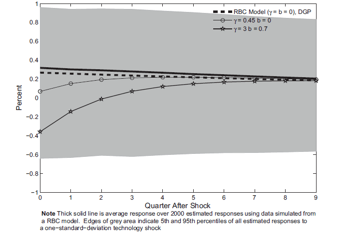
Figure 1 reports, for the benchmark VAR estimated using data simulated from a RBC model, the response of hours worked to a permanent shock to labor productivity with size equal to one-standard deviation. The gray area indicates the sampling distribution of the estimated impulse responses. The edges of the gray area indicate the 5th and 95th percentile of all the estimated impulse responses. These intervals are wide which is typical of structural VARs that are identified with a long-run restriction (see CEV 2006).
Figure 1 also reports the true impulse responses from several parameterizations of flexible price DSGE models that have real rigidities in the form of investment adjustment costs and habit persistence. These other responses all lie within the gray area, which, as previously mentioned, indicates sampling uncertainty. One, therefore, might be tempted to conclude that these impulse responses are unable to discriminate between the different parameterizations and, as such, that the statistical test of the hours response has poor power.9 The rest of this paper will show that a conclusion that these long-run VARs have poor power would be overly pessimistic.
Figure 2 reports a scatter plot of the estimated impact response of hours to a technology shock versus the corresponding estimated bootstrapped standard error for each of the 2000 simulations from the benchmark flexible price model. For any given simulation, we can determine whether an econometrician observing only that simulation would reject the true null hypothesis that the hours response on impact matches the response from a RBC model. If the econometrician had assumed that the estimated impulse response has an asymptotic normal distribution centered around the true response, then she would use a standard critical value of 2 and falsely reject the true null hypothesis 18 percent of the time. Given that the rejection rate is greater than the nominal size of 5 percent, we calculate the critical value (2.8), where an econometrician observing only a single data set would correctly fail to reject the null hypothesis 95 percent of the time and reject the true model only 5 percent of the time.10
5.1.1 Looking At Power
Figure 4 reports the same scatter plot of estimated impulse
responses and standard errors. However, Figure 4 reports the
results for testing whether the estimated impulse response matches
the response from a DSGE model with high levels of habit
![]() and investment
adjustment cost
and investment
adjustment cost
![]() . Even with the
size-corrected critical values, the false model is correctly
rejected 32 percent of the time. Using the standard critical value
would lead to an even greater rejection rate of 53 percent. These
results illustrate that one can find model parameterizations with
much higher rejections rates than the worse case that is analyzed
by Faust and Leeper.
. Even with the
size-corrected critical values, the false model is correctly
rejected 32 percent of the time. Using the standard critical value
would lead to an even greater rejection rate of 53 percent. These
results illustrate that one can find model parameterizations with
much higher rejections rates than the worse case that is analyzed
by Faust and Leeper.
Reporting the equivalent of Figure 4 for all possible
parameterizations is not feasible, as such, rejection rates are
summarized by Figure 5 which report for low degrees of habit
(Figure 5a) and high degrees of habit (Figure 5b), the rejection
rates for different values of ![]() The
rejection rates for the test of the impact response are indicated
by the solid lines and are labelled Sign, reflecting this
test's close relationship with previous papers that reported the
distribution of the sign of the impact response. When
The
rejection rates for the test of the impact response are indicated
by the solid lines and are labelled Sign, reflecting this
test's close relationship with previous papers that reported the
distribution of the sign of the impact response. When ![]() equals 0 and
equals 0 and ![]() equals 0, then the
rejection rate for the test of the impact response is the
likelihood of rejecting the true model and, as we are using a
size-corrected critical value, equals 5 percent by construction.
When
equals 0, then the
rejection rate for the test of the impact response is the
likelihood of rejecting the true model and, as we are using a
size-corrected critical value, equals 5 percent by construction.
When ![]() equals 3 and
equals 3 and ![]() equals
0.7, using the same size-corrected critical value, the rejection
rate is 32 percent.
equals
0.7, using the same size-corrected critical value, the rejection
rate is 32 percent.
As can be seen in Figure 5, the test is much more likely to
reject a false null hypothesis than a true null hypothesis. As
such, the evidence implies that, by restricting the model to a
plausible set of DSGE models, we gain power relative to the worse
case scenario of Faust and Leeper. Moreover, the rejection rates
increase with ![]() and
and ![]() However,
these rejection rates are not large. Even for parameterizations
with a fairly large degree of habit persistence and investment
adjustment costs, the test has a size-corrected rejection rate of
under 40 percent.
However,
these rejection rates are not large. Even for parameterizations
with a fairly large degree of habit persistence and investment
adjustment costs, the test has a size-corrected rejection rate of
under 40 percent.
To be able to discuss the usefulness of these long-run VARs, we need to determine whether the rejection rates reported in Figure 5 are high or low. Because statistical power is only infrequently reported, for comparison purposes, it would be useful to have a benchmark from the literature on statistical testing of DSGE models. One such statistic is the correlation of output growth.11 The inability of the RBC model to match the correlation of output growth has been an important statistic in casting doubt on the basic RBC model. Papers that discuss the correlation of output growth include Cogley and Nason (1995) and Christiano and Vigfusson (2003).
Results for this unconditional statistic help put the
performance of the impulse response analysis in context. Figure 5
also reports results for the output correlation (the dashed lines
labelled Correlation). Given the use of a size-corrected
critical value, the test of the correlation statistic rejects 5
percent of the time when ![]() and
and ![]() both equal zero. The power of these correlation statistics are
somewhat better than the impulse responses. The rejection rates
increase as both
both equal zero. The power of these correlation statistics are
somewhat better than the impulse responses. The rejection rates
increase as both ![]() and
and ![]() increase. With no habit persistence in consumption, the rejection
rates using the correlation are about 20 percent for models with
moderate or high degrees of investment adjustment costs
increase. With no habit persistence in consumption, the rejection
rates using the correlation are about 20 percent for models with
moderate or high degrees of investment adjustment costs ![]() . For models with a high degree of habit, the
correlations reject the false models much more frequently.
. For models with a high degree of habit, the
correlations reject the false models much more frequently.
Overall, this evidence suggests that the power of testing using the correlation is better than testing using just the impact response of hours worked. The rest of this paper shows that other applications of VARs can be more informative. In particular, Figure 5 has an additional set of lines that, for certain parameterizations, have better rejection rates than the rejection rates from the correlation test. The next section describes these lines.
5.2 Shape of Hours
In this section, we show that, compared to a test of the impact response, a test of the shape of the response of hours worked to a technology shock can more frequently reject false models. Studying the shape of impulse responses has a rich tradition in the empirical VAR literature. For example, based on VAR evidence, many variables respond with a delay to monetary policy shocks. To match these delayed responses, researchers abandoned frictionless, New-Classical models that implied immediate responses and adopted models with rigidities. (For a discussion of these issues, see Woodford 2003, p. 173).
Figure 6 reports, for data generated from a standard RBC model,
a scatter plot of the response of hours on impact and the change in
the response six periods later.12 Around each of these responses,
one could construct a confidence ellipse. Assuming that these
responses are drawn from a multivariate normal distribution, then
the formula for the confidence ellipse can be easily derived from a
simple Wald test. Given an estimated vector ![]() and a variance covariance matrix for
and a variance covariance matrix for
![]() denoted by
denoted by ![]() , then a point
, then a point ![]() lies in the 95
percent confidence ellipse if
lies in the 95
percent confidence ellipse if ![]() satisfies the
following inequality
satisfies the
following inequality
| (32) |
where ![]() is the critical value. According to
standard asymptotic theory, the statistic is distributed
chi-squared with 2 degrees of freedom. To estimate the
variance-covariance matrix
is the critical value. According to
standard asymptotic theory, the statistic is distributed
chi-squared with 2 degrees of freedom. To estimate the
variance-covariance matrix ![]() , weuse the
same method as we used to estimate the standard error. For each
simulated dataset, the variance-covariance matrix
, weuse the
same method as we used to estimate the standard error. For each
simulated dataset, the variance-covariance matrix ![]() is estimated using a bootstrap simulation where the
DGP is the estimated VAR using that specific dataset. As was done
for the impact responses, the test needs to be size-corrected. In
the simulations the value of
is estimated using a bootstrap simulation where the
DGP is the estimated VAR using that specific dataset. As was done
for the impact responses, the test needs to be size-corrected. In
the simulations the value of ![]() is 10
rather than the standard value of 6. To give some degree of the
magnitude of the correction, Figure 6 reports, for one single
simulation, the estimated confidence intervals using the two
different critical values. In either case, one would fail to reject
the true null hypothesis that the response matches the response
from the RBC model (the triangle). Although, the size-corrected
confidence set is much wider than the non-size corrected interval,
for this particular simulation, one would reject the false null
hypothesis that the response matches the response from a model with
high degrees of habit and investment adjustment costs (the square).
is 10
rather than the standard value of 6. To give some degree of the
magnitude of the correction, Figure 6 reports, for one single
simulation, the estimated confidence intervals using the two
different critical values. In either case, one would fail to reject
the true null hypothesis that the response matches the response
from the RBC model (the triangle). Although, the size-corrected
confidence set is much wider than the non-size corrected interval,
for this particular simulation, one would reject the false null
hypothesis that the response matches the response from a model with
high degrees of habit and investment adjustment costs (the square).
Returning to Figure 5, we can compare the power properties of the shape test versus the power properties of the tests of the impact response and the correlation. The rejection rates for tests using the shape of hours are much better than the rejection rates for tests using the sign and are comparable to rejection rates testing the correlation of output growth.
5.3 Investment Response
As was mentioned in CEV, the variance of hours explained by technology shocks is very low. In the benchmark parameterizations studied here, technology shocks account for less than 1 percent of the variance of hours. However, technology shocks do account for 22 percent of the variance of the ratio of investment to output. As such, a natural question to ask is whether looking at the response of investment rather than hours is more informative. We report below that the investment response does appear to be more informative.
Figure 6 plots the impulse responses estimated for investment from the same benchmark three variable VAR (with variables: labor productivity growth, hours worked and investment to output ratio). The various model responses again lie within the large gray area. Also of note is that, unlike with hours, the investment response is not monotonically increasing with respect to both habit and investment adjustment costs. For a given degree of habit persistence, the size of the investment response declines as the investment adjustment costs increase. However, for a high degree of habit persistence, the investment response is larger than would be the case with a low degree of habit. The economics behind this reversal is that, with a high degree of habit, the utility maximizing behavior is to invest more in order to smooth consumption.
Figure 7 reports the power properties of the two tests of investment and also reproduces from Figure 5 the rejection rates when one tests using the correlation of output, (the dashed lines). As indicated by the lines with circles, the shape of the investment response (again measured using the impact response and the response six periods later) seems more useful than the impact response (the solid line). Furthermore, both tests appear to be quite useful in discriminating between models.
5.4 Changing the True Data Generating Process
For the results reported above, the true data generating process is the RBC model. Given data simulated from the RBC model, we reported the rejection rate of the false null hypothesis that the data was generated from models with real rigidities. Of course, we are also interested in the opposite case where the data are simulated from a model with real rigidities and the false null hypothesis of the RBC model is tested. Reversing the role of the two models is particularly relevant as most empirical work favors models with various degrees of adjustment costs. (See ACEL and Smets and Wouters (2003) for examples).
For this exercise, we generate data from the model with high
investment adjustment costs and habit persistence with values of
![]() and
and ![]() set at the
values estimated in Christiano, Eichenbaum and Evans (2005). Using
data generated from this model, the statistical tests frequently
reject the standard RBC model. The rejection rates are much greater
than the rejection rates observed when data are simulated from the
RBC model and the test is of the model with high adjustment
costs.
set at the
values estimated in Christiano, Eichenbaum and Evans (2005). Using
data generated from this model, the statistical tests frequently
reject the standard RBC model. The rejection rates are much greater
than the rejection rates observed when data are simulated from the
RBC model and the test is of the model with high adjustment
costs.
Figure 8 reports the impulse response of hours worked. Given the high level of costs associated with adjusting either the level of consumption or investment, a technology shock actually drives down hours. The improvement in productivity causes the consumer to increase leisure rather than increase consumption or investment. The average estimated response is somewhat biased away from the true response. However, using the standard critical value, the rejection rate for testing the impact response compared to the true model impact response is 24 percent which is similar to the results presented above. As can be seen in Table 2, when using the size-corrected critical value, the power of the test to reject the impact response from the now false RBC model is 58 percent. Comparing these results with the results from Figure 5, the test of the impact response is much more powerful when the data are simulated from the model with real rigidities than when the data are simulated from the RBC model. Table 2 reports the power of testing the shape of the hours response using the size-adjusted critical values. By looking at the shape of the hours response, the false RBC model is rejected more than 90 percent of the time. Table 2 also reports the results for testing the investment response. For data simulated from this model with high real rigidities, as was the case for data simulated from the RBC model, the size and power properties are better for testing investment than testing hours. Using the investment response, one can almost always reject the RBC model. Finally Table 2 also reports a test using the correlation of output growth. Here too the statistic has a high degree of power.
Table 3 and Table 4 summarizes across several different parameterizations to reject the RBC model. For low levels of habit, testing the initial period of the hours response is not very informative but testing the shape of the hours response can be very informative. When there is no habit, the initial investment response is also not very informative. In models with a higher degree of habit, the initial investment response is much more informative.
Table 4 presents the values of the critical values that result in tests with correct size. For each test statistic, the critical values are fairly constant across parameterizations. As such, it seems reasonable to suppose that using the average critical value from this table is a good way to size correct when the true data generating process is unknown.
6. Simulation Results For Sticky Price Models
In this section, we present results for a model with sticky
prices with a moderate degree of price stickiness (
![]() , habit (b=0.4), and investment
adjustment costs (
, habit (b=0.4), and investment
adjustment costs (![]() . Given these model
parameters and other calibrated values reported in Table 1, we
estimated the sticky price model using the U.S. data. Using these
coefficient estimates which are also reported in Table 1, we
simulate data from this sticky price model and then look at
rejection rates for various models. In this section, we focus on
the Calvo adjustment parameter
. Given these model
parameters and other calibrated values reported in Table 1, we
estimated the sticky price model using the U.S. data. Using these
coefficient estimates which are also reported in Table 1, we
simulate data from this sticky price model and then look at
rejection rates for various models. In this section, we focus on
the Calvo adjustment parameter ![]() which
determines the degree of price stickiness.
which
determines the degree of price stickiness.
Table 5 reports results for a four variable VAR of labor
productivity growth, hours worked, the investment-to-output ratio
and real wages minus labor productivity (i.e. we impose the
cointegrated relationship between real wages and labor
productivity). As with the previous section, we did have some
problems with modest size distortion and, as such, had to increase
critical values to get the size of the test right, resulting in
wider confidence intervals. The rejection rates are reported for
various values of ![]() , which controls the
degree of price stickiness. Low values of
, which controls the
degree of price stickiness. Low values of ![]() are associated with less sticky prices.
are associated with less sticky prices.
High values of adjustment costs imply that regardless of the
degree of price stickiness, it is hard to differentiate amongst
models using data on either hours worked or investment adjustment
costs. The responses by hours worked and investment are similar for
high values of investment adjustment costs, regardless of the value
of ![]() or
or ![]() . One however, can
get better rejection rates by looking at wages. The rejection rates
are much higher for values of
. One however, can
get better rejection rates by looking at wages. The rejection rates
are much higher for values of ![]() that are far
from the true DGP.
that are far
from the true DGP.
The results from this section support the message from the previous section. In terms of discriminating amongst model parameterizations, it is best to examine those responses over which the parameterizations differ most. As such, to discriminate amongst models that differ in the degree of habit persistence or in the adjustment costs of investment, the investment response is most informative. To discriminate amongst models that differ to the degree of nominal rigidity, the wage response is most informative.
7. Empirical Application
As an empirical application, we take a VAR similar to that estimated in Christiano Eichenbaum and Vigfusson (2003) and ask what parameterizations can be ruled out and which can be allowed.
The VAR is the same three variable system used above in terms of labor productivity, hours worked and the ratio of investment to output. The difference is that rather than the data being simulated from a RBC model, the data are the empirical data from the United States. In particular, productivity is measured as hourly labor productivity in the business sector, hours worked is per capita business hours worked, and investment is the ratio of private nonresidential investment to GDP. In this section, hours enters the VAR in levels. The discussion of how to treat hours and other low frequency movements in estimating these VARs is beyond the scope of the current paper and is instead addressed in Christiano Eichenbaum and Vigfusson (2003). The sample period is 1954 to 2001.
Empirical responses are reported in Figure 9a, 9b, and 9c. In addition, for comparison sake, model impulse responses are reported for a few model parameterizations. A 95 percent confidence interval is constructed for the empirical responses using the estimated bootstrap error and a size-adjusted critical value that is the average of the values reported in Table 5. Given the width of the confidence interval, we fail to reject most of the models. We can reject the model with large real rigidities. However, models with only slightly less real rigidities would not be rejected. In contrast, Figure 10a, shows that, even when using the large size-adjusted critical value, a test based on the shape of the hours response does lead to a clear rejection of the large real rigidities. Likewise, the investment response leads us to reject a model with no real rigidities. Hence, although the sign is almost uninformative in this application, the shape of the responses is informative.
Based on these results, the most promising way to model the response to a technology shock is to allow for delayed hump-shaped responses to the technology shock. Future work will be directed towards determining whether these delayed responses are best modeled as the result of nominal or real rigidities.
8. Conclusions
Impulse responses from long-run VARs can reject false models. As expected, these rejection rates increase the further away the false model is from the true data-generating model. In addition, these rejection rates vary depending on what variables are studied. Overall, however, this paper shows that these long-run VARs can be informative about which models are to be preferred. For the models studied here, testing the shape is a more powerful test than simply looking at the sign of the response. In addition, relative to an alternative statistical test based on sample correlations, we find that the shape-based tests have greater power.
These results should encourage us to find creative and new ways to test our models. The conclusion is not to abandon our tools but to find ways to improve their use. Already several papers have explored methods to improve estimation with the long-run identification assumption including Feve and Guay (2009), Gospodinov (2008), Kascha and K. Mertens (2009), and E. Mertens (2008). Using these alternative methods, researchers may be able to improve on the results reported here. Overall, given these results on the power and size properties of long-run VARs, we conclude that these VARs can be useful for discriminating between macro models and, therefore, should continue to be used in developing and testing business cycle theory.
A. Understanding why the size correction is needed
To get the size correct, we need a larger critical value than has been used in applied literature. This section shows that this need for a larger-than-standard critical value is directly related to the persistence of hours worked. As has been discussed in the literature, the sampling properties of the impulse responses identified from a long-run VAR will be non-standard if hours worked has a unit root (CEV 2003) or near-unit root (Gospodinov 2008). Although hours worked is stationary in the RBC model, hours is highly persistent. In particular, consider the results from estimating the following covariate-augmented Dicky Fuller test which was featured in CEV.

where ![]() are other covariates. (in the
current application it is just productivity growth). An F-test of
whether
are other covariates. (in the
current application it is just productivity growth). An F-test of
whether ![]() equals zero is both a unit root test
and also a test of whether hours worked
equals zero is both a unit root test
and also a test of whether hours worked ![]() is a
weak instrument for hours growth
is a
weak instrument for hours growth
![]() 13
13
The top panel of Figure A reports the distribution of the f-test.14For most of the simulated data sets studied here, an econometrician would actually fail to reject the null hypothesis that hours worked is a weak instrument. The distribution of the F-test illustrates how the RBC model fails to model the dynamics in the actual U.S. data. In the actual U.S. data, the F-test has a value well about 10, which is quite unlikely for the RBC model. Hence, the average simulation from the RBC model is actually a much less suitable data generating process than is actual U.S. data for applying the long-run VAR estimation. Even though hours worked is persistent, first differencing hours does not solve the problem. As was shown before in EGG, CEV (2003) and CKM, first-differencing hours results in a very biased estimate of the hours response. As was documented in Gospodinov (2008), first-differencing hours can remove an important low frequency comovement between hours and labor-productivity growth. As such, even when hours is very persistent, estimating the VAR in levels works better than estimating the VAR with hours in first differences.
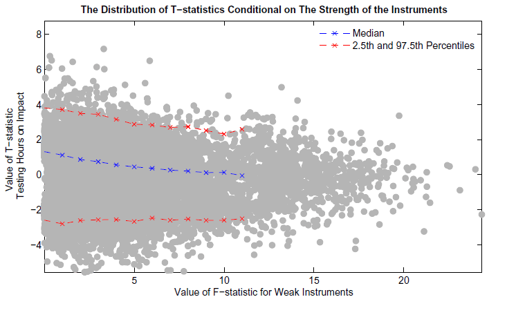
In the bottom panel, Figure A reports a scatter plot of the f-statistic for weak instruments relative to the t-statistic of testing the true hours response. Clearly the distribution of the t-statistic depends on the value of the f-statistic. Table A reports the ninety fifth percentile of the absolute value of the t-statistic conditioning on the value of the f-statistic. This table suggests a simple rule to correct the t-statistic. If the F-statistic is less than 10, then use a critical value of 3. If the F-statistic is more than 10, then use a critical value of 2. This simple rule of thumb approximates a more complex procedure that would adjust the confidence interval depending on the strength of the instruments.
References
Altig, David, Lawrence Christiano, Martin Eichenbaum, and Jesper Linde (2005). " Firm-Specific Capital, Nominal Rigidities, and the Business Cycle," NBER Working Paper Series 11034. Cambridge, Mass.: National Bureau of Economic Research, January.
Chari, V. V., Patrick J. Kehoe, and Ellen McGrattan (2008). " A Critique of Structural VARs Using Real Business Cycle Theory," Journal of Monetary Economics, vol. 55, pp. 1337-1352.
Christiano, Lawrence J., Martin Eichenbaum, and Charles Evans (2005). " Nominal Rigidities and the Dynamic Effects of a Shock to Monetary Policy," Journal of Political Economy, vol. 113 (February), pp. 1-45.
Christiano, Lawrence J., Martin Eichenbaum, and Robert Vigfusson (2003). " What Happens after a Technology Shock?" NBER Working Paper Series 9819. Cambridge, Mass.: National Bureau of Economic Research, July.
Christiano, Lawrence J., Martin Eichenbaum, and Robert Vigfusson (2006). " Assessing Structural VARS" NBER Macro Annual. Cambridge, Mass.: National Bureau of Economic Research.
Christiano Lawrence J. and Robert J. Vigfusson (2003) " Maximum likelihood in the frequency domain: the importance of time-to-plan", Journal of Monetary Economics, vol. 50, issue 4, pp. 789-815
Cogley, Timothy and Nason, James M, (1995). " Output Dynamics in Real-Business-Cycle Models," American Economic Review, vol. 85(3), June, pp. 492-511
Erceg, Christopher J., Luca Guerrieri, and Christopher Gust (2005). " Can Long-Run Restrictions Identify Technology Shocks?" Journal of the European Economic Association, vol. 3 (December), pp. 1237-78.
Erceg, Christopher J., Dale Henderson, and Andrew T. Levin, (2000). "Optimal monetary policy with staggered wage and price contracts," Journal of Monetary Economics, vol.46(2), pp. 281-313.
Faust, Jon (1999). " Conventional Confidence Intervals for Points on Spectrum Have Confidence Level Zero." Econometrica, vol 67(3), pp. 629-37.
Faust, Jon, and Eric Leeper (1997). " When Do Long-Run Identifying Restrictions Give Reliable Results?" Journal of Business and Economic Statistics, vol. 15 (July), pp. 345-53.
Fève, Partick and Alain Guay (2009) " Identification of Technology Shocks in Structural VARs" Economic Journal forthcoming
Francis, Neville, and Valerie A. Ramey (2005). " Is the Technology-Driven Real Business Cycle Hypothesis Dead? Shocks and Aggregate Fluctuations Revisited," Journal of Monetary Economics, vol. 52 (November), pp. 1379-99.
Gali, Jordi (1999). " Technology, Employment, and the Business Cycle: Do Technology Shocks Explain Aggregate Fluctuations?" American Economic Review, vol. 89 (March), pp. 249-71.
Gospodinov, Nikolay (2008). Inference in Nearly Nonstationary SVAR Models with Long-Run Identifying Restrictions Journal of Business and Economic Statistics forthcoming
Hamilton, James D. (1994). Time Series Analysis. Princeton: Princeton University Press.
Kascha Christian and Karel Mertens (2009) " Business Cycle Analysis and VARMA Models" Journal of Economic Dynamics and Control, 33(2), pp. 267-282
Kehoe Patrick J. (2006) " How to Advance Theory with Structural VARs: Use the Sims-Cogley-Nason Approach", NBER Macro Annual. Cambridge, Mass.: National Bureau of Economic Research.
Mertens Elmar (2008) " Are Spectral Estimators Useful for Implementing Long-Run Restrictions in SVARs?" manuscript
Sims, Christopher (1972). " The Role of Approximate Prior Restrictions in Distributed Lag Estimation," Journal of the American Statistical Association, vol. 67 (March), pp. 169-75.
Sims, Christopher and Tao Zha (2006) " Does Monetary Policy Generate Recessions?" Macroeconomic Dynamics, 10(2), pp. 231-72
Smets, Frank, and Raf Wouters (2003). " An Estimated Dynamic Stochastic General Equilibrium Model of the Euro Area," Journal of the European Economic Association, vol. 1 (September), pp. 1123-75.
Vigfusson, Robert J. (2004). " The Delayed Response to a Technology Shock: A Flexible Price Explanation," International Finance Discussion Paper Series 2004-810. Washington: Board of Governors of the Federal Reserve System, July.
Woodford, Michael M. (2003). Interest and Prices: Foundations of a Theory of Monetary Policy. Princeton: Princeton University Press.
Tables
Table 1a: Model Parameter Values - Calibrated
|
|
|
|
|
|
|
|
|
| |
|
Table 1b: Model Parameter Values - Estimated for Flexible Price Model
Table 1c: Model Parameter Values - Estimated for Sticky Price Model
Table 2: Size and Power when DGP is DSGE Model with High Adjustment Costs
| Test | Rejection Rate: RBC Model, Size Adjusted* | Rejection Rate: True Model, Not-size Adjusted | Critical Value |
|---|---|---|---|
| Impact Hours Response | 58 | 23 | 3.2 |
| Shape of Hours Response | 99 | 29 | 16.5 |
| Impact Investment Response | 100 | 10 | 2.4 |
| Shape of Investment Response | 100 | 13 | 9.84 |
| Correlation of Output Growth | 100 | 10 | 2.55 |
*Rejection Rates are for the size-adjusted critical values given in column (iii)
Table 3: Rejection Rates of the RBC Model (Percent)
| Model Parameters: b | Model Parameters: |
Test Statistic - Hours: Sign | Test Statistic - Hours: Shape | Test Statistic - Investment: Sign | Test Statistic - Investment: Shape | Test Statistic - Output: Correlation |
|---|---|---|---|---|---|---|
| 0 | 0.5 | 5 | 81 | 12 | 100 | 0 |
| 0 | 1.5 | 8 | 100 | 21 | 100 | 1 |
| 0 | 3 | 11 | 100 | 24 | 100 | 0 |
| 0.5 | 0.5 | 20 | 43 | 70 | 88 | 79 |
| 0.5 | 1.5 | 33 | 100 | 85 | 100 | 92 |
| 0.5 | 3 | 41 | 100 | 87 | 100 | 92 |
| 0.7 | 0.5 | 27 | 25 | 83 | 58 | 95 |
| 0.7 | 3 | 58 | 100 | 89 | 100 | 100 |
Results are reported for tests done on data simulated using the macro model described in the paper with parameters in the first two columns on the left. For each set of model parameters, 2000 simulations are done. For each parameterization, size-adjusted critical values are used to test the false null hypothesis that the data were generated by an RBC model.
Table 4: Size Adjusted Critical Values
| Model Parameters: b | Model Parameters: |
Test Statistic - Hours: Sign | Test Statistic - Hours: Shape | Test Statistic - Investment: Sign | Test Statistic - Investment: Shape | Test Statistic - Output: Correlation |
|---|---|---|---|---|---|---|
| 0 | 0 | 3.20 | 16.5 | 2.4 | 9.84 | 2.55 |
| 0 | 0.5 | 2.96 | 10.80 | 2.36 | 8.38 | 2.96 |
| 0 | 1.5 | 2.81 | 10.60 | 2.27 | 8.36 | 3.11 |
| 0 | 3 | 2.75 | 9.93 | 2.31 | 8.78 | 3.06 |
| 0.5 | 0.5 | 2.77 | 10.56 | 2.36 | 8.12 | 2.64 |
| 0.5 | 1.5 | 2.83 | 12.55 | 2.32 | 9.06 | 2.64 |
| 0.5 | 3 | 2.87 | 13.42 | 2.40 | 9.34 | 2.63 |
| 0.7 | 0.5 | 2.87 | 11.65 | 2.52 | 9.13 | 2.56 |
| 0.7 | 3 | 3.20 | 16.47 | 2.39 | 9.85 | 2.55 |
Table 5a: Rejection Rates (in Percent) For Various Degrees of Price Stickiness ![]() (Other Parameters b = 0.4 and
(Other Parameters b = 0.4 and ![]() )
)
| 0.15 | 0.35 | 0.55 | 0.75* | 0.9 | |
|---|---|---|---|---|---|
| Hours Impact | 2 | 2 | 3 | 5 | 8 |
| Hours Shape | 2 | 2 | 3 | 5 | 8 |
| Investment Impact | 5 | 5 | 5 | 5 | 8 |
| Investment Shape | 17 | 12 | 9 | 5 | 10 |
| Wage Impact | 32 | 20 | 11 | 5 | 4 |
| Wage Shape | 22 | 13 | 8 | 5 | 4 |
Table 5b: Rejection Rates (in Percent) For Various Degrees of Price Stickiness ![]() (Other Parameters b = 0.4 and
(Other Parameters b = 0.4 and ![]() )�
)�
| 0.15 | 0.35 | 0.55 | 0.75 | 0.9 | |
|---|---|---|---|---|---|
| Hours Impact | 9 | 3 | 11 | 100 | 100 |
| Hours Shape | 13 | 3 | 13 | 100 | 100 |
| Investment Impact | 73 | 27 | 19 | 100 | 100 |
| Investment Shape | 61 | 23 | 26 | 100 | 100 |
| Wage Impact | 24 | 17 | 6 | 29 | 94 |
| Wage Shape | 17 | 11 | 6 | 43 | 100 |
Table 5c: Rejection Rates (in Percent) For Various Degrees of Price Stickiness ![]() (Other Parameters b = 0.4 and
(Other Parameters b = 0.4 and![]() )�
)�
| 0.15 | 0.35 | 0.55 | 0.75 | 0.9 | |
|---|---|---|---|---|---|
| Hours Impact | 5 | 5 | 6 | 8 | 9 |
| Hours Shape | 5 | 5 | 6 | 7 | 9 |
| Investment Impact | 5 | 5 | 5 | 5 | 6 |
| Investment Shape | 19 | 13 | 10 | 8 | 9 |
| Wage Impact | 37 | 23 | 14 | 6 | 5 |
| Wage Shape | 27 | 16 | 10 | 6 | 4 |
* denotes DGP parameterization. Critical Values chosen to insure correct size.
Table A: Critical Values of The T-statistic of Impact Response of Hours conditional on a Test of Hours Being a Weak Instrument�
| F-statistic of Hours Being a Weak Instrument | Average Bias | Absolute Value of T-statistic 95th Percentile | Fraction of Observations (percent) |
|---|---|---|---|
| (0,1) | 1.31 | 3.12 | 15 |
| (1,2) | 1.12 | 3.15 | 14 |
| (2,3) | 0.87 | 2.96 | |
| (3,4) | 0.74 | 2.90 | 11 |
| (4,5) | 0.56 | 2.75 | 9 |
| (5,6) | 0.45 | 2.52 | 7 |
| (6,7) | 0.37 | 2.43 | 5 |
| (7,8) | 0.26 | 2.30 | 3 |
| (8,9) | 0.21 | 2.26 | 2 |
| (9,10) | 0.12 | 2.10 | 2 |
| (10,11) | 0.13 | 1.93 | 2 |
| (11,12) | -0.06 | 1.90 | 1 |
| -0.13 | 1.97 | 2 |
Figure 1: The response of hours worked to a technology shock estimated using data simulated from a RBC Model
Note: Thick solid line is average response over 2000 estimated responses using data simulated from a RBC model. Edges of grey area indicate 5th and 95th percentiles of all estimated responses to a one-standard-deviation technology shock.
Figure 2: Testing the Impact Repsonse of Hours
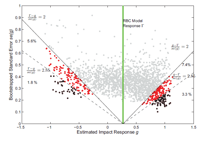
Figure 3: Testing the Impact Response of Hours using a false null hypothesis
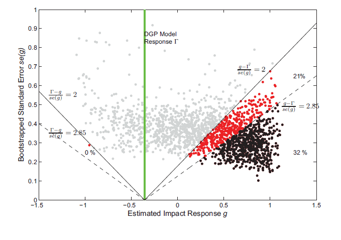
Figure 4: Rejection Rates for Different Tests when True GDP is RBC Model
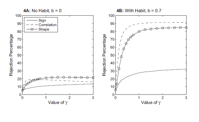
Figure 5: The Shape of Hours Response
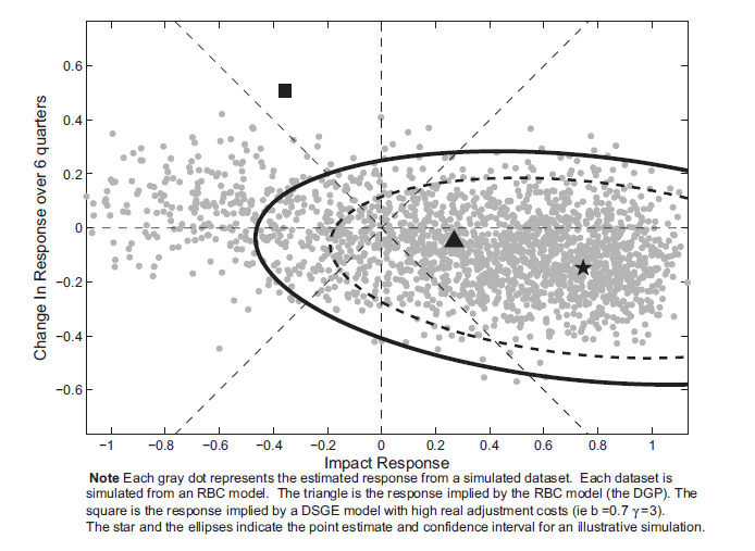
Note: Each gray dot represnets the estimated response from a simulated dataset. Each dataset is simulated from an RBC model. The triangle is the response implied by the RBC model (the DGP). The square is the response implied by a DSGE model with high real adjustment costs (ie b=0.7 γ=3). The star and the ellipses indicate the point estimate and confidence interval for an illustrative simulation.
Figure 6: The response of investment to a technology shock estimated using data simulated from a RBC Model
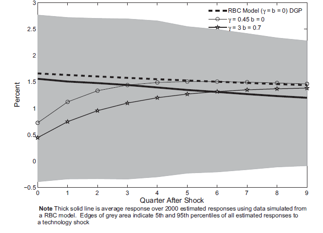
Note: Thick solid line is average response over 2000 estimated responses using data simulated from a RBC model. Edges of grey area indicate 5th and 95th percentiles of all estimated responses to a technology shock.
Figure 7: Rejection Rates for Testing Investment Response
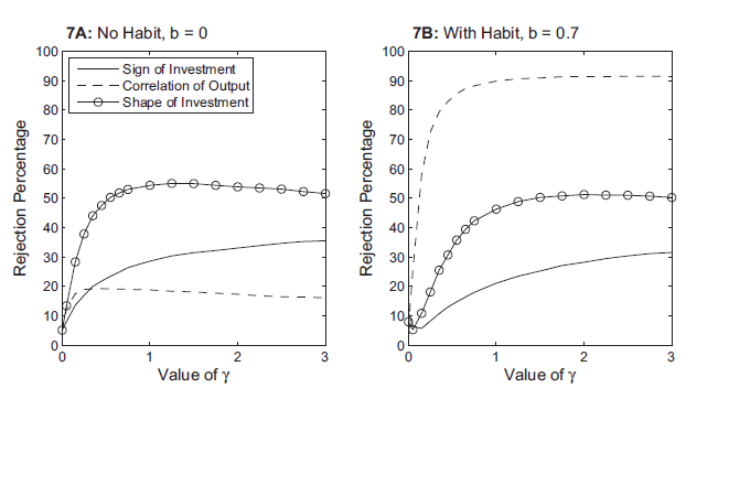
Figure 8: The response of hours worked to a technology shock estimated using data simulated from a model with high investment adj. costs and habit
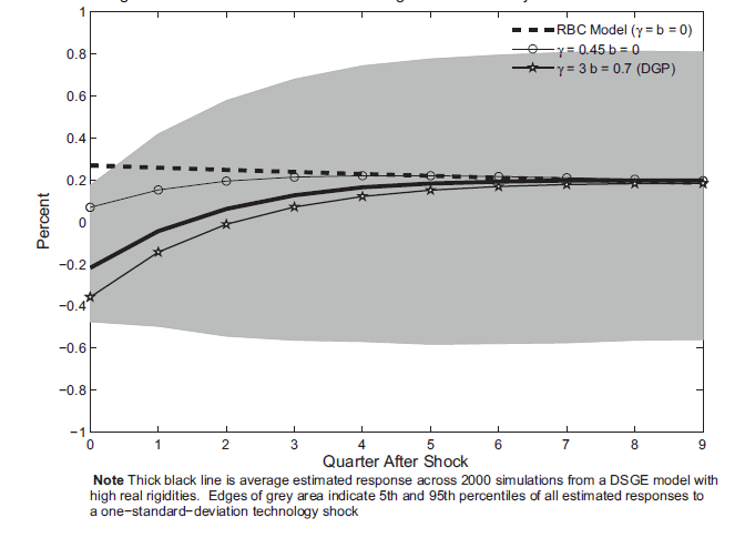
Note: Thick black line is average estimated response across 2000 simulations from a DSGE model with high real rigidities. Edges of grey area indicate 5th and 95th percentiles of all estimated responses to a one-standard-deviation technology shock.
Figure 9a: The estimated response of output to a technology process
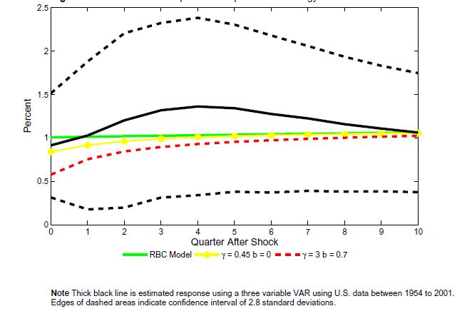
Note: Thick black line is estimated response using a three variable VAR using U.S. data between 1954 to 2001. Edges of dashed areas indicate confidence interval of 2.8 standard deviations.
Figure9b: The estimated response of hours worked to a technology shock

Note: Thick black line is estimated response using a three variable VAR using U.S. data between 1954 to 2001. Edges of dashed areas indicate confidence interval of 2.8 standard deviations.
Figure 9c: The estimated response of investment to a technology shock
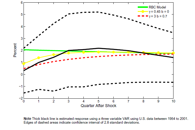
Note: Thick black line is estimated response using a three variable VAR using U.S. data between 1954 to 2001. Edges of dashed areas indicate confidence interval of 2.8 standard deviations.
Figure 10a: The Shape of the Hours response in an Estimated VAR
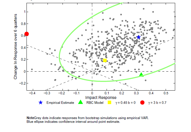
Note: Grey dots indicate responses from bootstrap simulations using empirical VAR. Blue ellipse indicates confidence interval around point estimate.
Figure 10b: The Shape of the Investment Response in an Estimated VAR
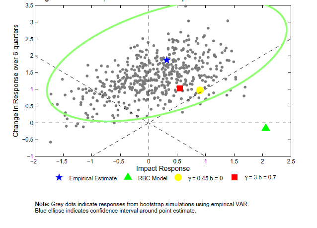
Note: Grey dots indicate responses from bootstrap simulations using empirical VAR. Blue ellipse indicates confidence interval around point estimate.
Figure A (top panel): Implications of Weak Instruments on Sampling Uncertainty - F Test for Weak Instruments
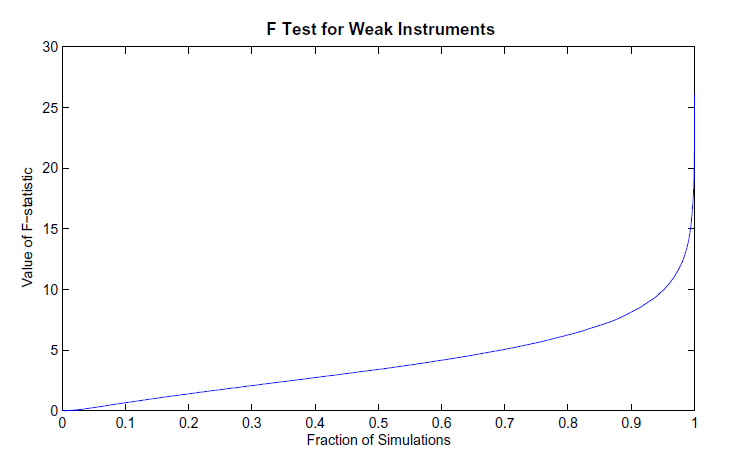
Figure A (bottom panel): Implications of Weak Instruments on Sampling Uncertainty - The Distribution of T-Statistics Conditional on the Strength of the Instruments
Footnotes
1. Thanks to Sylvain Leduc, Seth Pruitt, and Larry Christiano for comments. We also thank seminar participants at the Federal Reserve Board, the University of Manitoba, the Bank of Japan, the University of Tokyo, the University of Michigan, the SED Meetings, Midwest Macro Meetings, and Federal Reserve System's Macro Conference. The views in this paper are solely those of the authors and should not be interpreted as reflecting the views of the Board of Governors of the Federal Reserve System or of any other person associated with the Federal Reserve System. Return to text
2. Federal Reserve Board of Governors. Email: [email protected] Return to text
3. This result does not directly contradict Faust and Leeper as they themselves note that their proposition would be inapplicable if the set of DGPs was suitably restricted. For example, assuming that the DGP must be a finite-ordered VAR with maximum lag length K would be a sufficient restriction to make their proposition inapplicable. However, Faust and Leeper view such a restriction as being implausible. The current paper shows for the more plausible assumption that a macro model is the DGP, (which is an infinite-order VAR), then these long-run VARs do have power to reject false null hypothesis at a rate greater than the size of the test. Return to text
4. In the model that CKM studies, hours worked is stationary. In such a case, as is discussed in Christiano Eichenbaum and Vigfusson (2003), hours worked should enter the VAR in levels. Return to text
5. For convenience, we have suppressed the
state-dependent nature of
![]() . In equilibrium,
. In equilibrium,
![]() is equivalent to the price a
household pays for a claim in period
is equivalent to the price a
household pays for a claim in period ![]() that pays
one dollar if the corresponding state occurs in period
that pays
one dollar if the corresponding state occurs in period ![]() , normalized by the probability that state
occurs. Return to text
, normalized by the probability that state
occurs. Return to text
6. The constant term in the policy rule has been suppressed for simplicity. Return to text
7. When there are more shocks than variables, one can still derive a VAR. However, identifying all the shocks becomes more difficult. See Sims and Zha (2006) for more details. Return to text
8. The debate over using a finite VAR is present in the aforementioned EGG, CKM and CEV papers. Because of this debate, some have suggested estimating instead models with both autoregressive and moving average components (VARMA models). However, as was described in Kascha and K. Mertens (2009), the difficulties in estimating these VARMA models suggests that they do not offer much improvement. Return to text
9. The argument on page 1339 in CKM seems to be a claim of poor power. However, CKM never report the estimated statistical sampling uncertainty that a researcher would estimate when faced with only a single data set. Rather they just report the distribution of the point estimates. In terms of our Figure 2, they report the distribution of the values on the x-axis but do not calculate the values on the y-axis. Return to text
10. An alternative approach would be to experiment with the various proposed modifications of how to construct confidence intervals. However, as many different methods have been proposed, we leave explorations of the properties of these different methods for future work. Return to text
11. The confidence intervals for the
correlation statistic were constructed using the standard method
from the Matlab Statistics Toolbox. Confidence intervals were
constructed using the result that, for the correlation statistic
![]() the valu e of
the valu e of
![]() is
approximately normal with a variance equal to
is
approximately normal with a variance equal to
![]() . As with other statistics
reported in this paper, the critical value for testing the
correlation was size-corrected. Return
to text
. As with other statistics
reported in this paper, the critical value for testing the
correlation was size-corrected. Return
to text
12. The choice to looking at the response six periods later is somewhat arbitrary. One could imagine testing instead the period that creates the maximum change. However, a result-driven method such as this could result in exaggerating the response in a fashion analogous to the difference between a standard Chow test for parameter instability and the supremum Wald test of Andrews.
An additional extension would be to test the vector of responses between impact and many periods later. This route was not taken here in order to minimize the size of the V matrix that needed to be stored. However, an additional concern is that this larger test may be overly precisely and reject models that have the same rough shape as the empirical responses but that do not match period by period. Return to text
13. For VARs with more than two variables, we will have to use a multivariate test like the Cragg Donald test to assess the weakness of all the instruments. Return to text
14. These results are reported for 40,000 simulated data sets. Return to text
This version is optimized for use by screen readers. Descriptions for all mathematical expressions are provided in LaTex format. A printable pdf version is available. Return to text