
Board of Governors of the Federal Reserve System
International Finance Discussion Papers
Number 1053, August 2012 --- Screen Reader
Version*
Heterogeneous Workers, Optimal Job Seeking, and Aggregate Labor Market Dynamics
NOTE: International Finance Discussion Papers are preliminary materials circulated to stimulate discussion and critical comment. References in publications to International Finance Discussion Papers (other than an acknowledgment that the writer has had access to unpublished material) should be cleared with the author or authors. Recent IFDPs are available on the Web at http://www.federalreserve.gov/pubs/ifdp/. This paper can be downloaded without charge from the Social Science Research Network electronic library at http://www.ssrn.com/.
Abstract:
In the United States, the aggregate vacancy-unemployment (V/U) ratio is strongly procyclical, and a large fraction of its adjustment associated with changes in productivity is sluggish. The latter is entirely unexplained by the benchmark homogeneous-agent model of equilibrium unemployment theory. I show that endogenous search and worker-side horizontal heterogeneity in production capacity can be important in accounting for this propagation puzzle. Driven by differences in unemployed and on-the-job seekers' search incentives, the probability that any given firm with a job opening matches with a worker endowed with a comparative advantage in that job exhibits a stage of procyclical slow-moving adjustment. Consequently, so do the expected gains from posting vacancies and, hence, the V/U ratio. The model has channels through which the majority of both the V/U ratio's sluggish-adjustment properties and its elasticity with respect to output per worker can be accounted for.
Keywords: Amplification, comparative advantage, endogenous search, heterogeneity, market tightness, mismatch, on-the-job search, propagation, search and matching, search intensity, unemployment, vacancies
JEL classification: E25, J24, J64
1 Introduction
The aggregate vacancy-unemployment (V/U) ratio broadly summarizes the state of the labor market, as it reflects the ease with which individuals can exit unemployment. Empirically, in the United States, the V/U ratio is strongly procyclical, and a large fraction of its adjustment given changes in productivity is sluggish. Hence, for instance, an increase in productivity is associated with an upward jump in the V/U ratio, followed by a protracted stage over which the V/U ratio continues to slowly rise (at a decreasing rate). The benchmark, homogeneous-agent model of equilibrium unemployment theory has no channels through which such slow-moving adjustment can be accounted for: given a change in productivity, the model predicts that full adjustment of the V/U ratio occurs instantly. This limitation is additional to the well-known fact that under standard calibrations, the benchmark model can account for less than half of the elasticity of the V/U ratio with respect to productivity.1 Understanding the V/U ratio's stage of sluggish adjustment is important. Indeed, a slow-moving deterioration of the V/U ratio reflects the degree to which the labor market responds persistently, for example, in the wake of a recession. Moreover, as can be inferred from Fujita and Ramey (2007), around 60% of the total change in the V/U ratio that occurs given a change in productivity takes place during the V/U ratio's stage of sluggish adjustment.2
The objective of this paper is to develop an understanding of the extent to which endogenous search and horizontal worker-side heterogeneity in production capacity can have an impact on shaping the dynamic adjustment process of the V/U ratio relative to changes in productivity. I capture horizontal heterogeneity by considering a labor force composed of individuals who have a comparative advantage in a particular job, but are still able to work in jobs in which they have a comparative disadvantage. I assume no worker has an absolute advantage in production, and I endogenize the search behavior of all job seekers, both employed and unemployed, across all available job opportunities. The model I develop is not competing, but rather, complementary to the benchmark/standard model, which I show is nested within the present paper's framework.
Quantitative analysis reveals that the impact of horizontal worker-side heterogeneity and endogenous search can be substantial. Indeed, results imply that accounting for such factors can potentially help explain both the majority of the V/U ratio's slow-moving adjustment properties and the majority of its elasticity with respect to output per worker.
In the model, both workers and firms prefer comparative-advantage employment (matches between the same worker- and firm-type) over comparative-disadvantage employment (that is, matches between workers and firms whose type is different), since the former generates the highest surplus. Nonetheless, comparative disadvantage employment generates valuable surplus also; therefore, it represents an appealing alternative through which workers can exit unemployment, as well as an additional channel through which firms can fill positions and, accordingly, incur lower expected vacancy-posting costs. Given this environment, incentives are such that unemployed individuals search across all available job opportunities, and on-the-job (OTJ) search emerges naturally as the result of individuals who are employed in jobs in which they have a comparative disadvantage (alternatively, skill-mismatched employment), but search for comparative-advantage (alternatively, skill-matched) employment. The intensity of search that any given individual devotes to any given job opportunity is endogenous and contingent on: an individual's comparative advantage in production, the state of the economy, search costs, and an individual's employment state.
Given worker-side heterogeneity, vacancy-posting decisions are based on the expected value of a match, which depends on the slow-moving masses of unemployed and OTJ searchers. Consider, for example, an increase in productivity.3 This induces a sudden increase in the expected gains from posting vacancies, triggering a jump in the V/U ratio. Since unemployed individuals have a lower outside-search option compared to OTJ seekers, following the increase in productivity, as unemployment declines the ratio of OTJ searchers to unemployed individuals rises slowly. Consequently, the fraction of job seekers who direct search (exclusively) toward comparative-advantage employment opportunities increases. This leads to a slow-moving rise in the probability that any given firm with a job opening matches with a worker endowed with a comparative advantage in that job (that is, the probability that any given firm with a vacancy matches with a worker of its own type). Hence, the expected gains from posting vacancies exhibit a stage of sluggish increase, inducing the same in the V/U ratio. The opposite occurs in a contraction.
It follows that the process leading to slow-moving adjustment of the V/U ratio originates from endogenous changes in the composition of the pool of individuals searching for any particular type of job. Endogenous job-seeking magnifies this process and aids in accounting for the amplification of shocks by generating feedback between firm and worker-side decisions. In particular, this allows workers to respond optimally to relative changes in employment surpluses across job opportunities, which has a direct impact on cyclical changes in the composition of searchers, and hence, on firms' match-quality expectations.
As related to the role of worker-side heterogeneity, Albrecht and Vroman (2002), Gautier (2002), Chassamboulli (2009), and Dolado, Jansen, and Jimeno (2009) develop models that explore the impact of vertical worker-side skill differentiation on idiosyncratic differences in unemployment and wages, while Pries (2007) shows how vertical differentiation can help amplify aggregate productivity shocks. In turn, Bils, Chang, and Kim (2009) focus on understanding differences in unemployment and work hours across labor-force participants. In their analysis, worker-side heterogeneity operates in a context in which "comparative advantage" refers to individuals who have high market productivity relative to their home productivity. Furthermore, labor markets are segmented: although the labor force is heterogeneous, conditional on idiosyncratic characteristics individuals seek employment in only one production sector. In all of the previous, workers' search behavior is determined exogenously.
By accounting for horizontal worker-side differentiation and endogenous directed search, the analysis in the present paper complements the literature on three main fronts. First, it reveals the critical labor-market role of (directed) OTJ search. In the absence of this, workers' ability to refocus search given changes in productivity is limited to the extent that the model's channel for generating slow-moving adjustment of the V/U ratio is effectively shut down. Thus, comparative disadvantage employment emerges as necessary, but not sufficient for the V/U ratio to exhibit sluggish adjustment in response to changes in productivity. Second, analysis shows that the combination of worker-side heterogeneity and optimal search can generate amplification of changes in productivity broadly in line with the data even for relatively small values of net unemployment flow benefits. This stands in contrast to the fact that, as noted, for instance, in Hagedorn and Manovskii (2008), the standard model requires net unemployment flow benefits to be almost as large as output per worker in order to match the amplification of productivity shocks in the data. Finally, accounting for worker-side heterogeneity implies that output per worker (OPW) is endogenous. The theory reveals that, conditional on whether they stem from changes in productivity throughout or between job opportunities, otherwise identical changes in OPW can be associated with adjustment in aggregate labor-market variables of considerably different magnitude. Intuitively, changes in OPW that stem from changes in productivity between job opportunities are associated with greater changes in relative employment surpluses, and therefore with greater endogenous readjustment in the pool of individuals searching for any particular type of job.
This paper proceeds as follows. Section 2 develops the theory; although my ultimate interest lies in understanding the joint implications of worker-side heterogeneity and endogenous directed search, I develop the model sequentially, building it by initially focusing on the case in which search decisions are exogenous. Then, Section 3 details my methodology for numerical analysis, and Sections 4 and 5 present results. Finally, Section 6 concludes.
2 The Model
I consider an economy with two types of workers and two types of production sectors/firms, where worker-side differentiation is horizontal, and the environment is symmetric. This facilitates focus on developing an understanding of the extent to which arbitrarily small degrees of heterogeneity can have an impact on aggregate labor-market fluctuations relative to the standard, homogeneous-agent model of equilibrium unemployment theory.
I embed horizontal differentiation through assumptions on
production. Let workers and production sectors/firms be indexed by
![]() . In the notation subscripts
refer to workers and superscripts to sectors/firms. Comparative
advantage employment, which I alternatively refer to as
skill-matched employment, occurs when the worker and firm
type coincide. The output generated by a type-
. In the notation subscripts
refer to workers and superscripts to sectors/firms. Comparative
advantage employment, which I alternatively refer to as
skill-matched employment, occurs when the worker and firm
type coincide. The output generated by a type-![]() individual employed by a type-
individual employed by a type-![]() firm is
firm is
![]() , where
, where ![]() is an economy-wide (exogenous) productivity parameter.
For
is an economy-wide (exogenous) productivity parameter.
For ![]() , the output generated by a
type-
, the output generated by a
type-![]() individual employed by a type-
individual employed by a type-![]() firm (comparative disadvantage employment, or,
alternatively, skill-mismatched employment) is
firm (comparative disadvantage employment, or,
alternatively, skill-mismatched employment) is
![]() , where
, where
![]() is an (exogenous) penalty
parameter that captures the degree of comparative disadvantage of a
type-
is an (exogenous) penalty
parameter that captures the degree of comparative disadvantage of a
type-![]() individual employed by a type-
individual employed by a type-![]() firm. Unless noted otherwise, henceforth when
firm. Unless noted otherwise, henceforth when ![]() and
and ![]() appear together in some expression,
assume
appear together in some expression,
assume ![]() .
.
Symmetry implies that in all periods any type-specific
worker/firm variable is equal to half of its aggregate counterpart,
and that all model parameters are symmetric across worker and firm
types. Given symmetry, whenever helpful I present the model from
the point of view of type-1 economic agents. All statements carry
over to type-2 agents by simple re-indexing. As in Hagedorn and
Manovskii (2008) the model is cast in discrete time, but I assume
that the time period is small enough to be a close approximation to
continuous time. All economic agents discount the future at rate
![]() , and
, and
![]() is the discount
factor. In addition, all variables are normalized by the aggregate
labor force.
is the discount
factor. In addition, all variables are normalized by the aggregate
labor force.
Job seekers are in employment state
![]() , where
, where
![]() means " unemployed" and
means " unemployed" and ![]() means "skill-mismatch employed." Unemployed workers
receive net unemployment flow benefits
means "skill-mismatch employed." Unemployed workers
receive net unemployment flow benefits ![]() , which are
equal to the difference between time-invariant gross unemployment
flow benefits
, which are
equal to the difference between time-invariant gross unemployment
flow benefits ![]() and time-invariant (for now) search
costs
and time-invariant (for now) search
costs ![]() . Unemployed individuals direct their
search across all employment opportunities.4
. Unemployed individuals direct their
search across all employment opportunities.4
The value of unemployment for a type-1 individual is given by
![]() . All job-finding probabilities are
endogenous, and
. All job-finding probabilities are
endogenous, and
![]() denotes the
probability that a type-1 individual searching for a job in sector
denotes the
probability that a type-1 individual searching for a job in sector
![]() finds a job in that sector, given that he
or she is in employment state
finds a job in that sector, given that he
or she is in employment state
![]() . Moreover,
. Moreover,
![]() is the value of employment for a
type-1 individual who is matched with a type
is the value of employment for a
type-1 individual who is matched with a type ![]() firm. Letting
firm. Letting
![]() denote the expectation operator,
it follows that
denote the expectation operator,
it follows that
| |
(1) |
Comparative advantage in production implies that in any period
![]() . By assumption,
it is always true that
. By assumption,
it is always true that
![]() .
.
Let
![]() denote the wage of a type-1
individual who is matched with a type-
denote the wage of a type-1
individual who is matched with a type-![]() firm. As
noted in Shimer (2006), the standard Nash bargaining solution to
wage determination in matching models is invalid given on-the-job
search. Thus, in line with Pissarides (1994), Chassamboulli (2009),
and Dolado, Jansen, and Jimeno (2009), I assume that wages are such
that a constant fraction
firm. As
noted in Shimer (2006), the standard Nash bargaining solution to
wage determination in matching models is invalid given on-the-job
search. Thus, in line with Pissarides (1994), Chassamboulli (2009),
and Dolado, Jansen, and Jimeno (2009), I assume that wages are such
that a constant fraction ![]() of the surplus of a match
goes to the worker, where
of the surplus of a match
goes to the worker, where
![]() is the bargaining
power of workers,
is the bargaining
power of workers, ![]() goes to the firm, and
also that wages can be continuously revised and that long-term
contracts are not possible.5 Following the literature, there is an
exogenous job-destruction probability
goes to the firm, and
also that wages can be continuously revised and that long-term
contracts are not possible.5 Following the literature, there is an
exogenous job-destruction probability ![]() with which any type of job, whether skill-matched or -mismatched,
is destroyed. Since the value of skill-mismatch is less than that
of skill-matched employment, it is optimal for an individual who is
skill-mismatched to engage in on-the-job (OTJ) search directed
toward the sector in which he or she has a comparative advantage
(conditional on the type of match, the production functions of all
firms within a sector are identical, so there are no gains in
moving from one skill-mismatched employment relationship to
another). It follows that the value of comparative disadvantage
employment for a type-1 individual is
with which any type of job, whether skill-matched or -mismatched,
is destroyed. Since the value of skill-mismatch is less than that
of skill-matched employment, it is optimal for an individual who is
skill-mismatched to engage in on-the-job (OTJ) search directed
toward the sector in which he or she has a comparative advantage
(conditional on the type of match, the production functions of all
firms within a sector are identical, so there are no gains in
moving from one skill-mismatched employment relationship to
another). It follows that the value of comparative disadvantage
employment for a type-1 individual is
| |
(2) |
where ![]() represents (for now, time invariant)
OTJ search costs. Note that a job-to-job transition occurs with
probability
represents (for now, time invariant)
OTJ search costs. Note that a job-to-job transition occurs with
probability
![]() , meaning that there is an
endogenous job-destruction component associated with
skill-mismatched employment.
, meaning that there is an
endogenous job-destruction component associated with
skill-mismatched employment.
Using analogous reasoning, the relevant value of comparative advantage employment is
| (3) |
In this case, there is no endogenous job-destruction component, since skill-matched individuals have already achieved their best possible match. Hence, they do not engage in OTJ search.
Let ![]() ,
,
![]() and
and ![]() denote,
respectively, the mass of type-
denote,
respectively, the mass of type-![]() individuals who are
unemployed, skill-mismatch employed, and skill-match employed; each
of these masses is determined endogenously. Then,
individuals who are
unemployed, skill-mismatch employed, and skill-match employed; each
of these masses is determined endogenously. Then,
| (4) |
where, by symmetry,
![]() is the economy's fraction of
type-
is the economy's fraction of
type-![]() individuals.
individuals.
Each period, the number of matches formed in sector ![]() is determined by the sectoral matching function
is determined by the sectoral matching function
![]() , which is
increasing in sector-
, which is
increasing in sector-![]() vacancies
vacancies ![]() and searchers
and searchers ![]() . Following
related literature, such as Gautier (2002), I assume that
. Following
related literature, such as Gautier (2002), I assume that
![]() has constant returns to scale. In
particular, let
has constant returns to scale. In
particular, let
![]() , where
, where
![]() is the elasticity
of sectoral matches with respect to sectoral vacancies, and
is the elasticity
of sectoral matches with respect to sectoral vacancies, and
![]() is the matching efficiency parameter.
is the matching efficiency parameter.
The job-finding probability
![]() is given by
is given by
![]() (sector-
(sector-![]() matches per sector-
matches per sector-![]() searchers), weighted by the worker-type/employment-state specific
technological component
searchers), weighted by the worker-type/employment-state specific
technological component
![]() : effective
search. For now, I assume that effective search is determined
exogenously. Thus, in any period
: effective
search. For now, I assume that effective search is determined
exogenously. Thus, in any period
![]() . The
technological component of the search process summarizes the
effectiveness with which all of an individual's job-seeking
activities lead to a job offer given his or her employment state
and the sector in which the individual is searching.6
Effective search includes different kinds of search activities and
methods, the intensity with which search methods are used, etc. It
follows that sectoral searchers are a weighted sum of all
individuals searching in that sector, where the weights are
effective search. Thus, for instance,
. The
technological component of the search process summarizes the
effectiveness with which all of an individual's job-seeking
activities lead to a job offer given his or her employment state
and the sector in which the individual is searching.6
Effective search includes different kinds of search activities and
methods, the intensity with which search methods are used, etc. It
follows that sectoral searchers are a weighted sum of all
individuals searching in that sector, where the weights are
effective search. Thus, for instance,
| (5) |
Note that sector-1 searchers do not include the weighted mass of
skill-mismatched type-2 individuals
![]() , since
type-2 individuals who are employed in sector 1 only search for
sector-2 jobs.7 Given constant returns to scale
, since
type-2 individuals who are employed in sector 1 only search for
sector-2 jobs.7 Given constant returns to scale
![]() , where
, where
![]() denotes
sectoral (market) tightness, and
denotes
sectoral (market) tightness, and
![]() .
.
With the earlier development in mind, it is straightforward that
the evolution of the mass of unemployed type-![]() workers satisfies
workers satisfies
| (6) |
and the aggregate unemployment rate is
![]() . Moreover, the
evolution of the mass of type-
. Moreover, the
evolution of the mass of type-![]() workers who are
skill mismatched is given by
workers who are
skill mismatched is given by
| (7) |
with the aggregate rate of skill-mismatch satisfying
![]() . Finally,
letting
. Finally,
letting
![]() denote the
employment rate,
denote the
employment rate,
![]() is the aggregate rate of
skill-mismatched employment.
is the aggregate rate of
skill-mismatched employment.
Turning toward firms, let the value of a job for a sector-1 firm
that is matched with a type-![]() worker be denoted
by
worker be denoted
by
![]() , and the value of a vacancy by
, and the value of a vacancy by
![]() . The firm's value of skill-matched
employment is
. The firm's value of skill-matched
employment is
| (8) |
and its value of skill-mismatched employment is
| (9) |
Comparative advantage in production implies that
![]() .
.
Following the literature, while a firm has a vacancy it incurs
the time-invariant flow cost ![]() . The probability
with which a sector-
. The probability
with which a sector-![]() vacant job is filled is
vacant job is filled is
![]() (sector-
(sector-![]() matches per sector-
matches per sector-![]() vacancies). Given constant returns to scale, this can be stated as
vacancies). Given constant returns to scale, this can be stated as
![]() , where
, where
![]() . The probability that a
sector-
. The probability that a
sector-![]() vacant job is filled with a worker who has
a comparative advantage in that sector is
vacant job is filled with a worker who has
a comparative advantage in that sector is
![]() , and
, and
![]() otherwise. If follows
that
otherwise. If follows
that
| (10) |
and given the earlier development
 .
. |
(11) |
That is,
![]() is the effective fraction of
type-2 individuals looking for jobs in sector 1. This probability
is endogenous, and given its dependence on the slow-moving masses
of unemployed and OTJ searchers, slow moving as well. For short,
with some slight abuse of terminology, I henceforth refer to
is the effective fraction of
type-2 individuals looking for jobs in sector 1. This probability
is endogenous, and given its dependence on the slow-moving masses
of unemployed and OTJ searchers, slow moving as well. For short,
with some slight abuse of terminology, I henceforth refer to
![]() as the probability of
skill-mismatch.
as the probability of
skill-mismatch.
For
![]() ,
,
![]() is the surplus generated by an employment match between a
type-
is the surplus generated by an employment match between a
type-![]() worker and a sector-
worker and a sector-![]() firm. The earlier noted assumptions on wage negotiations jointly
imply that wages ultimately satisfy conditions identical to the
standard Nash bargaining solution, implying the surplus-sharing
rule
firm. The earlier noted assumptions on wage negotiations jointly
imply that wages ultimately satisfy conditions identical to the
standard Nash bargaining solution, implying the surplus-sharing
rule
| (12) |
Since
![]() (and
(and
![]() ), it follows that
), it follows that
![]() (and
(and
![]() ). Therefore, the
wage of an individual who is skill-mismatched is lower than his or
her skill-matched wage, and the wage of an individual who is
skill-mismatched in any given sector is lower than that of
individuals who are skill-matched in that same sector.
). Therefore, the
wage of an individual who is skill-mismatched is lower than his or
her skill-matched wage, and the wage of an individual who is
skill-mismatched in any given sector is lower than that of
individuals who are skill-matched in that same sector.
Free entry into vacancy creation implies the zero-profit
condition
![]() . Implementing this condition in
equation (10) along
with the definition of surplus and rearranging yields the
vacancy/job-creation condition:
. Implementing this condition in
equation (10) along
with the definition of surplus and rearranging yields the
vacancy/job-creation condition:
| (13) |
This is the model's fundamental equilibrium equation. Changes in
economy-wide productivity ![]() induce changes in
the expected gains from posting vacancies (the left-hand side
(LHS)). These changes must be balanced out in terms of changes in
expected costs (the right-hand side (RHS)). Such balancing occurs
through changes in
induce changes in
the expected gains from posting vacancies (the left-hand side
(LHS)). These changes must be balanced out in terms of changes in
expected costs (the right-hand side (RHS)). Such balancing occurs
through changes in ![]() , which is a decreasing
function of
, which is a decreasing
function of
![]() . It follows that
. It follows that
![]() and
and
![]() are the model's fundamental
equilibrium variables.8
are the model's fundamental
equilibrium variables.8
Henceforth, I refer to the model as developed so far, that is, with fixed effective search, as the multi-agent (MA) model.
2.1 The Role of Worker Heterogeneity
The MA model is not solvable analytically; however, the role of
worker heterogeneity can be understood intuitively by initially
focusing on the impact of the absence of heterogeneity.
Assume all workers are identical and normalize all production to
![]() . Then,
. Then,
![]() ,
,
![]() , and symmetry implies that
, and symmetry implies that
![]() , where
, where
![]() , and
additionally
, and
additionally ![]() , where
, where ![]() denotes
aggregate vacancies. Thus,
denotes
aggregate vacancies. Thus,
![]() , where
, where
![]() : the ratio of aggregate vacancies
to aggregate unemployment (alternatively, the V/U ratio). Hence,
: the ratio of aggregate vacancies
to aggregate unemployment (alternatively, the V/U ratio). Hence,
![]() , and, more
generally, super and subscripts become unnecessary since sectors
and individuals are now entirely identical. Within this context,
the job-creation condition reduces to
, and, more
generally, super and subscripts become unnecessary since sectors
and individuals are now entirely identical. Within this context,
the job-creation condition reduces to
| (14) |
which is, in fact, the standard (homogeneous agent) model's job creation condition.9 Thus, the standard model is a special case of the MA model in which heterogeneity is done away with.
Consider a permanent increase in economy-wide productivity
![]() . This leads to a one time, permanent
increase in the expected gains from posting vacancies (the LHS of
equation
. This leads to a one time, permanent
increase in the expected gains from posting vacancies (the LHS of
equation
![]() ) that is balanced out by a one-time increase in the expected costs
of posting vacancies (the equation's RHS). Since the job-filling
probability is a decreasing function of the V/U ratio, this
balancing occurs through a one-time increase in the V/U ratio,
which is driven by an instantaneous increase in aggregate
vacancies. Hence, given a change in
) that is balanced out by a one-time increase in the expected costs
of posting vacancies (the equation's RHS). Since the job-filling
probability is a decreasing function of the V/U ratio, this
balancing occurs through a one-time increase in the V/U ratio,
which is driven by an instantaneous increase in aggregate
vacancies. Hence, given a change in ![]() , the V/U
ratio does not exhibit post-shock slow-moving adjustment.
, the V/U
ratio does not exhibit post-shock slow-moving adjustment.
Now, return to the MA model, and once again consider a permanent
increase in ![]() . At the moment of the shock, the
expected gains from posting vacancies jump up (the LHS of equation
(13), as do
the expected costs (the equation's RHS). The latter is driven by an
instantaneous increase in sectoral market tightness
. At the moment of the shock, the
expected gains from posting vacancies jump up (the LHS of equation
(13), as do
the expected costs (the equation's RHS). The latter is driven by an
instantaneous increase in sectoral market tightness
![]() , which itself is driven by a jump
in sectoral vacancies. However, unlike the standard model, all
adjustments do not end there. This is because the probability of
skill-mismatch
, which itself is driven by a jump
in sectoral vacancies. However, unlike the standard model, all
adjustments do not end there. This is because the probability of
skill-mismatch
![]() is slow moving, and therefore,
only after the change in productivity has occurred will this
probability begin to adjust. By extension, the expected gains from
posting vacancies will also continue to (slowly) adjust after the
change in
is slow moving, and therefore,
only after the change in productivity has occurred will this
probability begin to adjust. By extension, the expected gains from
posting vacancies will also continue to (slowly) adjust after the
change in ![]() .
.
When economy-wide productivity rises, as the pool of unemployed
individuals declines, type-![]() workers take
relatively longer to exit
workers take
relatively longer to exit ![]() than
type-
than
type-![]() searchers. This is because upon becoming
skill-mismatched, type-
searchers. This is because upon becoming
skill-mismatched, type-![]() individuals become OTJ
searchers, and therefore continue to form part of
individuals become OTJ
searchers, and therefore continue to form part of ![]() ; however, type-
; however, type-![]() workers exit
workers exit
![]() whether they become skill-matched or
-mismatched. Such relatively faster drainage of type-
whether they become skill-matched or
-mismatched. Such relatively faster drainage of type-![]() workers maps into a decrease in the probability of
skill-mismatch
workers maps into a decrease in the probability of
skill-mismatch
![]() , which occurs slowly given its
dependence on the slow-moving masses of unemployed and OTJ
searchers. This leads to a slow-moving increase in the expected
gains from posting vacancies, which is balanced out through a
slow-moving increase in the expected costs, driven by a slow-moving
increase in sectoral market tightness. By extension, the
slow-moving increase in the availability of sectoral vacancies per
searchers will lead to a slow-moving increase in the availability
of aggregate vacancies per unemployed individual. Thus, in the MA
model, an increase in economy-wide productivity results in a stage
of slow-moving increase in the V/U ratio, with the reverse being
true given a decline in
, which occurs slowly given its
dependence on the slow-moving masses of unemployed and OTJ
searchers. This leads to a slow-moving increase in the expected
gains from posting vacancies, which is balanced out through a
slow-moving increase in the expected costs, driven by a slow-moving
increase in sectoral market tightness. By extension, the
slow-moving increase in the availability of sectoral vacancies per
searchers will lead to a slow-moving increase in the availability
of aggregate vacancies per unemployed individual. Thus, in the MA
model, an increase in economy-wide productivity results in a stage
of slow-moving increase in the V/U ratio, with the reverse being
true given a decline in ![]() .
.
More technically, note that given symmetry equation (11) can be stated as
 .
. |
(15) |
As such, the expression for
![]() clearly shows that in an
expansion it is a slow-moving increase in the ratio of
skill-mismatched employment to unemployment that serves to foster a
slow-moving decline in the probability of skill-mismatch. Note, in
addition, that in the absence of OTJ search
clearly shows that in an
expansion it is a slow-moving increase in the ratio of
skill-mismatched employment to unemployment that serves to foster a
slow-moving decline in the probability of skill-mismatch. Note, in
addition, that in the absence of OTJ search
![]() , and therefore
, and therefore
![]() reduces to being a constant,
meaning that the model's channel for generating sluggish adjustment
of the V/U ratio is effectively shut down.10
reduces to being a constant,
meaning that the model's channel for generating sluggish adjustment
of the V/U ratio is effectively shut down.10
The employment surpluses associated with skill-matched and -mismatched employment can be expressed, in steady state, respectively as
| (16) |
and
| (17) |
The term
![]() in equation
(16) and its
analog in equation
(17) capture,
respectively, the opportunity costs of skill-matched and
-mismatched employment.11 As detailed in the appendix, a
permanent increase in relative productivity
in equation
(16) and its
analog in equation
(17) capture,
respectively, the opportunity costs of skill-matched and
-mismatched employment.11 As detailed in the appendix, a
permanent increase in relative productivity ![]() induces an on impact decrease in the expected gains
from posting vacancies. Intuitively, this reflects the relative
importance of skill-matched surplus in firms' vacancy-posting
decisions, and therefore, the extent to which a weighing down of
the highest surplus-generating employment arrangement in the
economy - due to higher opportunity costs - is particularly
damaging for overall vacancy-posting incentives. It follows that in
the MA model a decrease in
induces an on impact decrease in the expected gains
from posting vacancies. Intuitively, this reflects the relative
importance of skill-matched surplus in firms' vacancy-posting
decisions, and therefore, the extent to which a weighing down of
the highest surplus-generating employment arrangement in the
economy - due to higher opportunity costs - is particularly
damaging for overall vacancy-posting incentives. It follows that in
the MA model a decrease in ![]() will induce the
economy to adjust opposite to an increase in economy-wide
productivity
will induce the
economy to adjust opposite to an increase in economy-wide
productivity ![]() , ultimately triggering a decline in
the V/U ratio, part of which will be slow-moving. The reverse will
occur given a decline in
, ultimately triggering a decline in
the V/U ratio, part of which will be slow-moving. The reverse will
occur given a decline in ![]() .
.
2.2 The Role of Optimal Effective Search
The costs of effective search directed toward a sector are simply the costs of generating job offers in that sector. As noted in Krueger and Mueller (2008), the time that unemployed individuals spend searching is small, which suggests that time constraints are not binding in optimal search decisions.12 Given this, an intuitive reason for which unemployed individuals might limit the effective search that they devote to any given type of job opportunity is that search costs are sector specific. In turn, sector-specific search costs are a natural motivation for individuals to broaden their search to include jobs in which they do not have a comparative advantage. To capture this intuition, I assume that individuals bear the additively separable effective-search disutility function
 ,
, |
(18) |
where
![]() .
.
Of course, the only value functions that must be updated are a
workers' value of skill-mismatched employment and unemployment.
Quite simply,
![]() and
and ![]() are as
before, except that now they are maximized, respectively, over
are as
before, except that now they are maximized, respectively, over
![]() , and
, and
![]() and
and
![]() . Moreover, net
unemployment flow benefits become endogenous, since
. Moreover, net
unemployment flow benefits become endogenous, since ![]() is now equal to the difference between
is now equal to the difference between ![]() and
and ![]() . As before, I assume that in all
states of the economy it is optimal for unemployed individuals to
search for jobs across sectors. Given the surplus-sharing rule in
equation
(12) , the first-order conditions for optimal search can be stated
as
. As before, I assume that in all
states of the economy it is optimal for unemployed individuals to
search for jobs across sectors. Given the surplus-sharing rule in
equation
(12) , the first-order conditions for optimal search can be stated
as
| (19) |
when skill-mismatched, and for
![]()
| (20) |
when unemployed.13 In each of these first-order conditions the RHS represents the expected gains from search. Note that effective search is a jump variable.
The intuitive nature of the cost function is reflected on
several fronts. By symmetry
![]() . Therefore, since
. Therefore, since
![]() , given equation
(20) unemployed individuals will always devote greater effective search
toward skill-matched employment:
, given equation
(20) unemployed individuals will always devote greater effective search
toward skill-matched employment:
![]()
![]() . This implies self selection.
Furthermore, if non-symmetric environments were considered, the
chosen cost function provides an additional and natural motivation
for skill-mismatched employment to exist. Suppose
. This implies self selection.
Furthermore, if non-symmetric environments were considered, the
chosen cost function provides an additional and natural motivation
for skill-mismatched employment to exist. Suppose ![]() . Then, it is optimal to set
. Then, it is optimal to set
![]() , but as long as the
expected gains from skill-mismatched search are positive
, but as long as the
expected gains from skill-mismatched search are positive
![]() .
.
I henceforth refer to the MA model extended to account for endogenous effective search as the multi-agent optimal search (MA-OS) model. This is the paper's central model of interest.
The MA-OS model nests three models. These are the MA model
(obtained by fixing effective search), the standard model (obtained
by fixing effective search and setting ![]() ), and a
version of the standard model in which effective search is
endogenous (standard optimal search (standard-OS) model; set
), and a
version of the standard model in which effective search is
endogenous (standard optimal search (standard-OS) model; set
![]() , but allow unemployed individuals to
choose effective search). Given the absence of worker-side
heterogeneity (and OTJ search), as is the case with the standard
model, the standard-OS model has no channels through which sluggish
adjustment of the V/U ratio can be generated.14
, but allow unemployed individuals to
choose effective search). Given the absence of worker-side
heterogeneity (and OTJ search), as is the case with the standard
model, the standard-OS model has no channels through which sluggish
adjustment of the V/U ratio can be generated.14
Related literature focuses on the response of models' endogenous
variables relative to changes in output per worker (OPW). In the
case of the standard and standard-OS models, OPW corresponds in
straightforward fashion to the exogenous economy-wide productivity
parameter ![]() . In contrast, in the MA and MA-OS
models OPW is determined endogenously, and given by
. In contrast, in the MA and MA-OS
models OPW is determined endogenously, and given by
| (21) |
Equation
(21) calls
explicit attention to the role of both economy-wide productivity
![]() and the skill-mismatch parameter
and the skill-mismatch parameter
![]() in the determination of OPW. This
highlights the fact that observed empirical changes in OPW need not
stem from a unique source.
in the determination of OPW. This
highlights the fact that observed empirical changes in OPW need not
stem from a unique source.
Although the MA-OS model is not solvable analytically, the
impact of endogenous effective search can still be gauged. Since
employment surpluses are procyclical in ![]() , then so are
the expected gains from search, and therefore, effective search as
well (recall equations
(19) and
(20)).
Intuitively, in an expansion jobs are easier to find and employment
surpluses are higher. This means that the opportunity cost of not
having a job, and for that matter, of being skill-mismatched,
increases. Hence, individuals react to above-average economic
conditions by supplying above-average effective search. In a
recession, the opposite occurs. For instance, think of discouraged
workers as an extreme example of this; these are individuals who
have set effective search equal to zero.15
, then so are
the expected gains from search, and therefore, effective search as
well (recall equations
(19) and
(20)).
Intuitively, in an expansion jobs are easier to find and employment
surpluses are higher. This means that the opportunity cost of not
having a job, and for that matter, of being skill-mismatched,
increases. Hence, individuals react to above-average economic
conditions by supplying above-average effective search. In a
recession, the opposite occurs. For instance, think of discouraged
workers as an extreme example of this; these are individuals who
have set effective search equal to zero.15
Endogenous effective search enhances the amplification of
economy-wide productivity shocks because it generates feedback
between firm- and worker-side decisions. For instance, when the
expected gains from search increase, effective search rises, which
decreases expected vacancy-posting costs (all else equal,
![]() declines). This raises the
expected gains from posting vacancies, therefore increasing
vacancies, which raises the expected gains from search, and so on
and so forth.
declines). This raises the
expected gains from posting vacancies, therefore increasing
vacancies, which raises the expected gains from search, and so on
and so forth.
Endogenous effective search also enhances the magnitude of the
model's sluggish adjustment properties. This is so because it
induces greater adjustment in the ratio of skill-mismatched
employment ![]() . Indeed, since employed job
seekers have a more attractive outside option than unemployed ones,
which is employment itself, it follows that unemployed effective
search is more procyclical than OTJ search (mathematically,
contrast equation
(20) to
equation
(19)).
Hence, in response to a rise in economy-wide productivity the
probability of entering skill-mismatched employment will increase
relatively more than the probability of exiting skill-mismatched
employment. This will magnify the post shock increase in
. Indeed, since employed job
seekers have a more attractive outside option than unemployed ones,
which is employment itself, it follows that unemployed effective
search is more procyclical than OTJ search (mathematically,
contrast equation
(20) to
equation
(19)).
Hence, in response to a rise in economy-wide productivity the
probability of entering skill-mismatched employment will increase
relatively more than the probability of exiting skill-mismatched
employment. This will magnify the post shock increase in
![]() relative to the MA model, and,
accordingly, the post shock decline in the probability of
skill-mismatch
relative to the MA model, and,
accordingly, the post shock decline in the probability of
skill-mismatch
![]() . Note that regardless of any
jump in
. Note that regardless of any
jump in
![]() , it is the slow-moving changes
of this variable that matter for sluggish adjustment of the V/U
ratio. Therefore, the magnified slow-moving decrease in
, it is the slow-moving changes
of this variable that matter for sluggish adjustment of the V/U
ratio. Therefore, the magnified slow-moving decrease in
![]() that occurs under endogenous
search will accordingly enhance the slow-moving adjustment of the
V/U ratio. Of course, in terms of both amplification and sluggish
adjustment, a decline in
that occurs under endogenous
search will accordingly enhance the slow-moving adjustment of the
V/U ratio. Of course, in terms of both amplification and sluggish
adjustment, a decline in ![]() will induce opposite
effects to those detailed above.
will induce opposite
effects to those detailed above.
Now, consider instead the effects of a permanent increase in
![]() . Recall from analysis of the MA model
that this will induce a reduction in the expected gains from
posting vacancies. In the MA-OS model, this effect will be
amplified because on impact of the the increase in
. Recall from analysis of the MA model
that this will induce a reduction in the expected gains from
posting vacancies. In the MA-OS model, this effect will be
amplified because on impact of the the increase in ![]() there will be an accompanying strong instantaneous
increase in the relative effective search that unemployed
individuals devote to comparative disadvantage employment. This, of
course, will lead to an instantaneous increase in the probability
of skill-mismatch, further depressing the expected gains from
posting vacancies.
there will be an accompanying strong instantaneous
increase in the relative effective search that unemployed
individuals devote to comparative disadvantage employment. This, of
course, will lead to an instantaneous increase in the probability
of skill-mismatch, further depressing the expected gains from
posting vacancies.
However, the extent to which greater relative effective search
devoted to skill-mismatched employment leads to (slow-moving)
increases in the ratio of skill-mismatched employment to
unemployment ![]() implies that following an
increase in
implies that following an
increase in ![]() the probability of skill-mismatch
will slowly decrease (recall, once more, equation
(15)). In
response to this, the V/U ratio will slowly rise. Hence, once
effective search is endogenized, an increase in
the probability of skill-mismatch
will slowly decrease (recall, once more, equation
(15)). In
response to this, the V/U ratio will slowly rise. Hence, once
effective search is endogenized, an increase in ![]() can in fact lead to an overall increase in the ratio
of aggregate vacancies to unemployment, reversing the associated
implications noted earlier for the MA model.
can in fact lead to an overall increase in the ratio
of aggregate vacancies to unemployment, reversing the associated
implications noted earlier for the MA model.
In addition, in the MA-OS model, because an increase in
![]() induces a relatively greater increase
in effective search devoted toward skill-mismatched employment than
an increase in
induces a relatively greater increase
in effective search devoted toward skill-mismatched employment than
an increase in ![]() (which has a direct and broad
impact across all effective search), the ratio
(which has a direct and broad
impact across all effective search), the ratio ![]() will (slowly) increase more following the former than
following the latter. Given equation
(15),
this implies that changes in
will (slowly) increase more following the former than
following the latter. Given equation
(15),
this implies that changes in ![]() will tend to
induce greater slow-moving adjustment of the V/U ratio than changes
in
will tend to
induce greater slow-moving adjustment of the V/U ratio than changes
in ![]() . Moreover, it also follows that changes in
. Moreover, it also follows that changes in
![]() will tend to have less of an impact
on OPW than changes in
will tend to have less of an impact
on OPW than changes in ![]() . Indeed, note from equation
(21) that
while an increase in
. Indeed, note from equation
(21) that
while an increase in ![]() , all else equal, tends
to increase OPW, a relative increase in
, all else equal, tends
to increase OPW, a relative increase in ![]() , all else
equal, tends to decrease OPW. In contrast, an increase in
, all else
equal, tends to decrease OPW. In contrast, an increase in
![]() works broadly toward increasing OPW
through increases in both skill-matched and -mismatched
productivity. Of course, a decline in
works broadly toward increasing OPW
through increases in both skill-matched and -mismatched
productivity. Of course, a decline in ![]() induces
opposite effects to those stemming from an increase in relative
productivity.
induces
opposite effects to those stemming from an increase in relative
productivity.
3 Basis for Numerical Analysis of Permanent Shocks
My analysis will focus on the impact of permanent changes in
models' exogenous variables, as this substantially simplifies the
explanation and interpretation of results while fully addressing
the issues of central interest.16 In order to gain a full
understanding of the MA-OS model, in analogous fashion to earlier
in the paper, numerical analysis will contrast results to those
stemming from nested models. There are no empirical time-series
counterparts to the parameters ![]() and
and ![]() ; therefore, following related literature, results are
put in context by highlighting changes in endogenous variables
relative to changes in output per worker, when relevant. All
henceforth cited tables and figures can be found in the
appendix.
; therefore, following related literature, results are
put in context by highlighting changes in endogenous variables
relative to changes in output per worker, when relevant. All
henceforth cited tables and figures can be found in the
appendix.
The choice of parameter values for each model is summarized in
Table 1. I assume that the time period is equal to one week.
Accordingly, I set the discount factor ![]() to
0.999, which is consistent with a quarterly
interest rate of 0.012. I use the matching function efficiency
parameter
to
0.999, which is consistent with a quarterly
interest rate of 0.012. I use the matching function efficiency
parameter ![]() and the flow cost of vacancy posting
and the flow cost of vacancy posting
![]() to target the equilibrium aggregate
unemployment rate
to target the equilibrium aggregate
unemployment rate ![]() and the equilibrium
V/U ratio
and the equilibrium
V/U ratio
![]() ; this is in line with averages
of US data spanning the last six decades. Using US unemployment
data and the methodology described in Shimer (2005), I obtain the
job-finding probability of an average unemployed individual. At
monthly frequency, the mean of this is equal to 0.43. The associated job-finding probability at weekly
frequency is given by
; this is in line with averages
of US data spanning the last six decades. Using US unemployment
data and the methodology described in Shimer (2005), I obtain the
job-finding probability of an average unemployed individual. At
monthly frequency, the mean of this is equal to 0.43. The associated job-finding probability at weekly
frequency is given by
![]() , which is
equal to 0.131; I take this as the relevant
steady-state value. Using this and the target equilibrium
unemployment rate, solving for the exogenous job-destruction
probability implies
, which is
equal to 0.131; I take this as the relevant
steady-state value. Using this and the target equilibrium
unemployment rate, solving for the exogenous job-destruction
probability implies
![]() .17 In all cases, the
matching function exponent
.17 In all cases, the
matching function exponent ![]() is chosen so
that the partial elasticity of aggregate matches with respect to
aggregate unemployment is in line with the corresponding evidence
from Petrongolo and Pissarides (2001).18
is chosen so
that the partial elasticity of aggregate matches with respect to
aggregate unemployment is in line with the corresponding evidence
from Petrongolo and Pissarides (2001).18
The parameters ![]() and
and
![]() are specific to the MA-OS and
standard-OS models. Numerical analysis reveals that for each
are specific to the MA-OS and
standard-OS models. Numerical analysis reveals that for each
![]() there is a value of
there is a value of ![]() that will hit the target equilibrium unemployment rate, but nothing
else changes. Thus, I normalize
that will hit the target equilibrium unemployment rate, but nothing
else changes. Thus, I normalize ![]() by setting
this parameter equal to one. In addition, I assume quadratic
effective search disutility, meaning that
by setting
this parameter equal to one. In addition, I assume quadratic
effective search disutility, meaning that
![]() .
.
The skill-mismatch parameter ![]() is specific to
the MA and MA-OS models. McLaughlin and Bils (2001) argue that
average within-industry wage differentials between individuals who
remain in an industry and those who switch can be interpreted as
the result of equilibrium self-selection. They show that,
empirically, the wages of industry switchers are, on average, 16
lower than those of industry non-switchers. I take this number as a
reference point. Therefore, I use the skill-mismatch penalty
parameter
is specific to
the MA and MA-OS models. McLaughlin and Bils (2001) argue that
average within-industry wage differentials between individuals who
remain in an industry and those who switch can be interpreted as
the result of equilibrium self-selection. They show that,
empirically, the wages of industry switchers are, on average, 16
lower than those of industry non-switchers. I take this number as a
reference point. Therefore, I use the skill-mismatch penalty
parameter ![]() to set the equilibrium ratio of
wages of skill-mismatched individuals to average wages in a sector
equal to 0.84.
to set the equilibrium ratio of
wages of skill-mismatched individuals to average wages in a sector
equal to 0.84.
In the case of the MA model, effective search is assumed to be
fixed at the equilibrium values implied endogenously by the MA-OS
model. In order to further tighten the comparability of results, I
purge the analysis from cross-model imbalances in bargaining power
by setting the parameter ![]() equal to 0.5. In
addition, I anchor all models around a common value for net
unemployment flow benefits
equal to 0.5. In
addition, I anchor all models around a common value for net
unemployment flow benefits ![]() , which I set to
0.5. This is the average of the values
advanced in Shimer (2005) and Hall and Milgrom (2008), assuming, in
the latter, the lowest suggested replacement rate. Anchoring around
, which I set to
0.5. This is the average of the values
advanced in Shimer (2005) and Hall and Milgrom (2008), assuming, in
the latter, the lowest suggested replacement rate. Anchoring around
![]() is in line with the fact that it is the
value of
is in line with the fact that it is the
value of ![]() , not
, not ![]() , which matters
directly for the determination of the value of employment surpluses
(recall equations
(16) and
(17)).
, which matters
directly for the determination of the value of employment surpluses
(recall equations
(16) and
(17)).
In all cases, the initial steady state of models is calculated
at ![]() . Numerical analysis reveals that in the
MA and MA-OS models the fraction of skill-mismatched employment is
always small, making the equilibrium value of output per worker
(OPW) arbitrarily close to one. Thus, across models, equilibrium
net unemployment flow benefits are approximately 50% of
OPW.19
. Numerical analysis reveals that in the
MA and MA-OS models the fraction of skill-mismatched employment is
always small, making the equilibrium value of output per worker
(OPW) arbitrarily close to one. Thus, across models, equilibrium
net unemployment flow benefits are approximately 50% of
OPW.19
4 Results I: Permanent Increases in Productivity
Figures 1 through 6 focus on the response of key endogenous
variables to a 1 permanent (unanticipated) increase in economy-wide
productivity ![]() . As shown in Figure 1, in the standard
model on impact of the shock
. As shown in Figure 1, in the standard
model on impact of the shock ![]() instantaneously jumps to its new equilibrium value, while in the
MA-OS model
instantaneously jumps to its new equilibrium value, while in the
MA-OS model ![]() initially jumps, and thereafter
continues to slowly increase over 4 months. This slow-moving
increase in the V/U ratio is driven by the slow-moving post-shock
decline in the probability of skill-mismatch
initially jumps, and thereafter
continues to slowly increase over 4 months. This slow-moving
increase in the V/U ratio is driven by the slow-moving post-shock
decline in the probability of skill-mismatch
![]() shown in Figure 2, which stems
from the slow-moving post-shock increase in the ratio of
skill-mismatched to unemployed individuals
shown in Figure 2, which stems
from the slow-moving post-shock increase in the ratio of
skill-mismatched to unemployed individuals ![]() shown in Figure 3 (recall equation
(15)).
shown in Figure 3 (recall equation
(15)).
In the MA-OS model
![]() . The jump in
. The jump in
![]() noted in Figure 2 is driven by
the greater procyclicality of effective search devoted to
skill-mismatched jobs (U
noted in Figure 2 is driven by
the greater procyclicality of effective search devoted to
skill-mismatched jobs (U
![]() skill-mismatch,
skill-mismatch,
![]() ,
, ![]() )
relative to unemployed and OTJ effective search devoted to
skill-matched search (U
)
relative to unemployed and OTJ effective search devoted to
skill-matched search (U
![]() skill-match,
skill-match,
![]() , and OTJ search,
, and OTJ search,
![]() , respectively); this is
shown in Figure 4, and stems from the expected gains from search
for skill-mismatched employment always being relatively
lower.20 The relatively greater
procyclicality of
, respectively); this is
shown in Figure 4, and stems from the expected gains from search
for skill-mismatched employment always being relatively
lower.20 The relatively greater
procyclicality of
![]() also accounts for the
relative adjustments in the slow-moving components of the
probability of skill-mismatch, as shown in Figure 5 (given symmetry
the percent changes in
also accounts for the
relative adjustments in the slow-moving components of the
probability of skill-mismatch, as shown in Figure 5 (given symmetry
the percent changes in ![]() and
and ![]() are the same as those in their aggregate
counterparts), and that of the fraction of skill-mismatched
employment
are the same as those in their aggregate
counterparts), and that of the fraction of skill-mismatched
employment ![]() is shown in Figure 6.
is shown in Figure 6.
Figures 7 and 8 show the individual responses of aggregate
vacancies, ![]() , and unemployment,
, and unemployment, ![]() .
In both models, on impact of the shock vacancies overshoot. In
terms of the response of the V/U ratio, the key difference is that
while in the standard model after the shock takes place vacancies
decline at the same rate that unemployment does, in the MA-OS model
the post-shock slow-moving decline in the probability of
skill-mismatch maintains incentives for vacancy posting higher than
otherwise. Hence, in the MA-OS model, after their initial jump
vacancies decrease, but at a slower rate relative to unemployment
than in the absence of a post-shock decline in the probability of
skill-mismatch.
.
In both models, on impact of the shock vacancies overshoot. In
terms of the response of the V/U ratio, the key difference is that
while in the standard model after the shock takes place vacancies
decline at the same rate that unemployment does, in the MA-OS model
the post-shock slow-moving decline in the probability of
skill-mismatch maintains incentives for vacancy posting higher than
otherwise. Hence, in the MA-OS model, after their initial jump
vacancies decrease, but at a slower rate relative to unemployment
than in the absence of a post-shock decline in the probability of
skill-mismatch.
Of course, in the standard model the elasticity of OPW with
respect to ![]() is one. In the MA-OS model, the 1%
change in economy-wide productivity under consideration induces a
1.003% change in OPW. As shown in Figure 6, in the MA-OS model a
permanent increase in
is one. In the MA-OS model, the 1%
change in economy-wide productivity under consideration induces a
1.003% change in OPW. As shown in Figure 6, in the MA-OS model a
permanent increase in ![]() ultimately induces a
decline in the fraction of skill-mismatched employment
ultimately induces a
decline in the fraction of skill-mismatched employment ![]() . Hence, in terms of OPW, the change in
. Hence, in terms of OPW, the change in ![]() is slightly amplified.
is slightly amplified.
Figures 9 through 16 focus on the response of key endogenous
variables to a 1% (unexpected) permanent increase in ![]() in the MA-OS model. As shown in Figure 9, while on
impact of the shock the V/U ratio declines, thereafter it slowly
increases across a period of roughly 15 months over which it fully
reverses its initial decline, ultimately increasing relative to its
starting value. Figures 10 and 11 show the corresponding changes in
aggregate vacancies and unemployment. Of course, the on-impact
decline in
in the MA-OS model. As shown in Figure 9, while on
impact of the shock the V/U ratio declines, thereafter it slowly
increases across a period of roughly 15 months over which it fully
reverses its initial decline, ultimately increasing relative to its
starting value. Figures 10 and 11 show the corresponding changes in
aggregate vacancies and unemployment. Of course, the on-impact
decline in ![]() is driven by an on-impact decline
in vacancies, which now exhibit a stage of sluggish adjustment.
Indeed, after their initial jump, vacancies slowly increase in the
direction of change of the exogenous driving force.
is driven by an on-impact decline
in vacancies, which now exhibit a stage of sluggish adjustment.
Indeed, after their initial jump, vacancies slowly increase in the
direction of change of the exogenous driving force.
Figure 12 shows adjustment in the probability of skill-mismatch
![]() . Its initial jump, along with
its persistent post-shock direction of change, is driven by the
initial response of endogenous effective search. As shown in Figure
13, on impact of the increase in
. Its initial jump, along with
its persistent post-shock direction of change, is driven by the
initial response of endogenous effective search. As shown in Figure
13, on impact of the increase in ![]() the
associated increase in skill-mismatched employment surplus triggers
a substantial increase in effective search devoted to such jobs,
partially at the expense of that devoted to skill-matched
employment. Figure 14 details the ensuing changes in the rate of
skill-mismatch
the
associated increase in skill-mismatched employment surplus triggers
a substantial increase in effective search devoted to such jobs,
partially at the expense of that devoted to skill-matched
employment. Figure 14 details the ensuing changes in the rate of
skill-mismatch ![]() and the ratio of
skill-mismatched employment to unemployment
and the ratio of
skill-mismatched employment to unemployment ![]() .
Overall, it follows that the lack of propagation slow-moving
vacancies response given changes in economy-wide productivity
.
Overall, it follows that the lack of propagation slow-moving
vacancies response given changes in economy-wide productivity
![]() , as shown earlier, is simply a reflection
of accompanying changes in the probability of skill-mismatch not
being sufficiently large.
, as shown earlier, is simply a reflection
of accompanying changes in the probability of skill-mismatch not
being sufficiently large.
As shown in Figure 15, unsurprisingly, the increase in
![]() induces a substantial increase in the
fraction of skill-mismatched employment,
induces a substantial increase in the
fraction of skill-mismatched employment, ![]() .
In terms of OPW, the relative increase in skill-mismatched
employment acts opposite to the increase in relative productivity
.
In terms of OPW, the relative increase in skill-mismatched
employment acts opposite to the increase in relative productivity
![]() . This leads, in particular, to the
elasticity of OPW with respect to
. This leads, in particular, to the
elasticity of OPW with respect to ![]() to be a
meager 0.002. Overall, the analysis reveals that once endogenous
effective search is accounted for, changes in relative productivity
have the potential to be a much more powerful driving force than
economy-wide productivity
to be a
meager 0.002. Overall, the analysis reveals that once endogenous
effective search is accounted for, changes in relative productivity
have the potential to be a much more powerful driving force than
economy-wide productivity ![]() in terms of both
amplification and propagation of shocks in the model's key
endogenous variables.
in terms of both
amplification and propagation of shocks in the model's key
endogenous variables.
5 Results II: Permanent Increases in OPW
Following related literature, I now focus on changes in models'
endogenous variables relative to changes in OPW.21 In
addition, I extend the analysis to account for the impact of joint
changes in ![]() and
and ![]() . In particular,
I focus on joint shocks in which both economy-wide and relative
productivity move in the same direction. This is intuitive given
that in the MA-OS model the (unique) skill-mismatched employment
opportunity is a stand-in for all jobs other than the one in
which a worker is most productive. Therefore, to the extent that an
increase in
. In particular,
I focus on joint shocks in which both economy-wide and relative
productivity move in the same direction. This is intuitive given
that in the MA-OS model the (unique) skill-mismatched employment
opportunity is a stand-in for all jobs other than the one in
which a worker is most productive. Therefore, to the extent that an
increase in ![]() represents an increase in a
worker's outside option relative to skill-matched employment, an
increase in
represents an increase in a
worker's outside option relative to skill-matched employment, an
increase in ![]() occurring jointly with an
increase in
occurring jointly with an
increase in ![]() is broadly analogous to it being the
case that in an expansion individuals have relatively more
viable work opportunities available than otherwise.
is broadly analogous to it being the
case that in an expansion individuals have relatively more
viable work opportunities available than otherwise.
Row R1 of Table 2 summarizes information stemming from empirical
US data. The elasticities of the V/U ratio ![]() ,
aggregate vacancies
,
aggregate vacancies ![]() , and aggregate unemployment
, and aggregate unemployment
![]() with respect to OPW are, respectively,
7.79, 3.88, and -3.93 (columns C1, C4, C7). Moreover, the
elasticity of vacancies with respect to unemployment, which
implicitly captures the slope of the Beveridge curve, that is, the
empirical negative relationship between aggregate vacancies and
unemployment, is -0.86 (column C9).22 Turning toward the
propagation of productivity shocks, some broadly applicable
stylized facts can be inferred from the detailed analysis in Fujita
and Ramey (2007). These are summarized in columns C2, C3, C5, C6,
and C8. Empirically, in the United States, an impulse in OPW of
around 0.7% is associated with: 1) an on-impact jump in the V/U
ratio that is followed by a stage of slow-moving increase (that
occurs at a decreasing rate) during which approximately 60% of the
total rise in the V/U ratio takes place (the V/U ratio peaks around
12 months after the increase in OPW occurs), 2) a (decreasing rate)
decline in the aggregate unemployment rate that lasts approximately
15 months before bottoming out, and 3) sluggishness in the
adjustment of vacancies; on impact vacancies jump, and thereafter
they continue to rise (at a decreasing rate) for about 12 months
over which approximately 60% of their total increase occurs. It
follows that, empirically, slow-moving adjustment of vacancies is
an important contributing factor to the sluggish adjustment of the
V/U ratio.
with respect to OPW are, respectively,
7.79, 3.88, and -3.93 (columns C1, C4, C7). Moreover, the
elasticity of vacancies with respect to unemployment, which
implicitly captures the slope of the Beveridge curve, that is, the
empirical negative relationship between aggregate vacancies and
unemployment, is -0.86 (column C9).22 Turning toward the
propagation of productivity shocks, some broadly applicable
stylized facts can be inferred from the detailed analysis in Fujita
and Ramey (2007). These are summarized in columns C2, C3, C5, C6,
and C8. Empirically, in the United States, an impulse in OPW of
around 0.7% is associated with: 1) an on-impact jump in the V/U
ratio that is followed by a stage of slow-moving increase (that
occurs at a decreasing rate) during which approximately 60% of the
total rise in the V/U ratio takes place (the V/U ratio peaks around
12 months after the increase in OPW occurs), 2) a (decreasing rate)
decline in the aggregate unemployment rate that lasts approximately
15 months before bottoming out, and 3) sluggishness in the
adjustment of vacancies; on impact vacancies jump, and thereafter
they continue to rise (at a decreasing rate) for about 12 months
over which approximately 60% of their total increase occurs. It
follows that, empirically, slow-moving adjustment of vacancies is
an important contributing factor to the sluggish adjustment of the
V/U ratio.
Rows R2 through R5 in Table 2 show model-specific responses to a
![]() -induced on-impact increase in OPW of 0.7%,
broadly serving to summarize results already shown in Section 4, and also, for comparison, incorporating
results pertaining to the standard-OS and MA models.23 The
standard model has limited explanatory power, accounting, in
particular, for 27% of the empirical elasticity of the V/U ratio
with respect to OPW, but none of its sluggish adjustment. The MA
model accounts for a similar fraction of the empirical elasticity
of the V/U ratio, but its dynamic adjustment is fundamentally
different than in the standard model, as it is characterized by a
stage of slow-moving response induced by vacancies adjusting at a
slower rate than unemployment. Comparatively similar are the
relative responses in the standard-OS and MA-OS models, with the
former accounting for 55% of the empirical elasticity of
-induced on-impact increase in OPW of 0.7%,
broadly serving to summarize results already shown in Section 4, and also, for comparison, incorporating
results pertaining to the standard-OS and MA models.23 The
standard model has limited explanatory power, accounting, in
particular, for 27% of the empirical elasticity of the V/U ratio
with respect to OPW, but none of its sluggish adjustment. The MA
model accounts for a similar fraction of the empirical elasticity
of the V/U ratio, but its dynamic adjustment is fundamentally
different than in the standard model, as it is characterized by a
stage of slow-moving response induced by vacancies adjusting at a
slower rate than unemployment. Comparatively similar are the
relative responses in the standard-OS and MA-OS models, with the
former accounting for 55% of the empirical elasticity of
![]() with respect to OPW, and the latter
for 64%. The last column of Table 2 (C10) shows the elasticity of
OPW with respect to the initial impulse of the relevant
exogenous driving force(s).
with respect to OPW, and the latter
for 64%. The last column of Table 2 (C10) shows the elasticity of
OPW with respect to the initial impulse of the relevant
exogenous driving force(s).
It follows that limiting changes in OPW to being driven by
changes in ![]() , relative to all other models MA-OS
makes the most important gains in accounting for sluggish
adjustment of
, relative to all other models MA-OS
makes the most important gains in accounting for sluggish
adjustment of ![]() , with its post-shock stage of
slow-moving adjustment lasting for 4 months over which 12% of its
total increase occurs. Thus, in response to a
, with its post-shock stage of
slow-moving adjustment lasting for 4 months over which 12% of its
total increase occurs. Thus, in response to a ![]() -induced increase in OPW, the MA-OS model's slow-moving
adjustment properties are approximately 25% of its empirical
counterparts. Moreover, as noted above, the model accounts for
around 2/3 of the empirical elasticity of the V/U ratio with
respect to OPW. Overall, results highlight the extent to which
endogenous effective search aids in accounting for the
amplification of productivity shocks, worker-side heterogeneity
aids with propagation, and the combination of both magnifies their
individual effects.
-induced increase in OPW, the MA-OS model's slow-moving
adjustment properties are approximately 25% of its empirical
counterparts. Moreover, as noted above, the model accounts for
around 2/3 of the empirical elasticity of the V/U ratio with
respect to OPW. Overall, results highlight the extent to which
endogenous effective search aids in accounting for the
amplification of productivity shocks, worker-side heterogeneity
aids with propagation, and the combination of both magnifies their
individual effects.
Figures 16 through 20 show responses in the MA-OS model's key
endogenous variables to joint increases in ![]() and
and
![]() that (in all cases) induce an
on-impact increase in OPW of 0.7%, where the size of the shock to
that (in all cases) induce an
on-impact increase in OPW of 0.7%, where the size of the shock to
![]() is, alternatively, half of the shock
in
is, alternatively, half of the shock
in ![]() , equal to the shock in
, equal to the shock in ![]() ,
and two, three, four, and five times the shock in
,
and two, three, four, and five times the shock in ![]() (the legend in Figure 16 applies to Figures 17 through 20). For
reference, the noted set of figures also shows the case
corresponding to row R5 of Table 2, which is the situation in which
only a shock in
(the legend in Figure 16 applies to Figures 17 through 20). For
reference, the noted set of figures also shows the case
corresponding to row R5 of Table 2, which is the situation in which
only a shock in ![]() occurs.
occurs.
Figure 16 highlights that the greater the contribution of
relative productivity to the shock, the greater the total response
of the V/U ratio, as well as the magnitude of the extent to which
it adjusts sluggishly. Moreover, when combined with an increase in
economy-wide productivity, an increase in ![]() does not necessarily induce an on-impact decrease in the V/U ratio,
as shown earlier to be the case given a stand-alone increase in
does not necessarily induce an on-impact decrease in the V/U ratio,
as shown earlier to be the case given a stand-alone increase in
![]() . As shown in Figure 17, this carries
over to vacancies; moreover, while vacancies do not exhibit
sluggish adjustment for relatively small changes in
. As shown in Figure 17, this carries
over to vacancies; moreover, while vacancies do not exhibit
sluggish adjustment for relatively small changes in ![]() , they do for higher ones. Figure 18 shows the
corresponding changes in unemployment, and Figure 19 shows changes
in
, they do for higher ones. Figure 18 shows the
corresponding changes in unemployment, and Figure 19 shows changes
in ![]() ; greater and longer increases in
; greater and longer increases in
![]() are associated with greater and
longer post-shock decreases in the the probability of
skill-mismatch, which induces greater and longer post shock
increases in the V/U ratio. Finally, Figure 20 shows the relevant
adjustments in the fraction of skill-mismatched employment
are associated with greater and
longer post-shock decreases in the the probability of
skill-mismatch, which induces greater and longer post shock
increases in the V/U ratio. Finally, Figure 20 shows the relevant
adjustments in the fraction of skill-mismatched employment
![]() .
.
Rows R6 through R11 of Table 2 put in context the information
shown in Figures 16 through 20. As the relative contribution of
![]() to the rise in OPW increases, the
MA-OS model makes substantial progress in broadly accounting for
the entirety of the US empirical data, both in terms of
amplification and propagation of productivity shocks. This is
particularly important on four fronts. First, the fact that the
model is capable of generating sluggish adjustment of both the V/U
ratio and vacancies implies substantial improvement relative to the
standard model, which has no channels through which this can occur.
Second, it is noteworthy that the MA-OS model can yield
amplification broadly in line with the data, as captured by the
elasticities noted in Table 2, even for relatively small values of
net unemployment flow benefits. This stands in contrast to the fact
that, as noted, for instance, in Hagedorn and Manovskii (2008), the
standard model requires net unemployment flow benefits to be almost
as large as OPW in order to match the amplification of productivity
shocks in the data.24 Third, results highlight that, given
heterogeneity, not all productivity shocks induce equivalent
dynamic adjustments. In particular, the model suggests that changes
in relative productivity are a key factor driving observed changes
in aggregate labor-market variables. Finally, it is particularly
noteworthy that even in the absence of changes in relative
productivity, the MA-OS model already makes substantial progress in
accounting for both amplification and propagation of productivity
shocks relative to the standard model, as noted earlier in row R5
of Table 2.
to the rise in OPW increases, the
MA-OS model makes substantial progress in broadly accounting for
the entirety of the US empirical data, both in terms of
amplification and propagation of productivity shocks. This is
particularly important on four fronts. First, the fact that the
model is capable of generating sluggish adjustment of both the V/U
ratio and vacancies implies substantial improvement relative to the
standard model, which has no channels through which this can occur.
Second, it is noteworthy that the MA-OS model can yield
amplification broadly in line with the data, as captured by the
elasticities noted in Table 2, even for relatively small values of
net unemployment flow benefits. This stands in contrast to the fact
that, as noted, for instance, in Hagedorn and Manovskii (2008), the
standard model requires net unemployment flow benefits to be almost
as large as OPW in order to match the amplification of productivity
shocks in the data.24 Third, results highlight that, given
heterogeneity, not all productivity shocks induce equivalent
dynamic adjustments. In particular, the model suggests that changes
in relative productivity are a key factor driving observed changes
in aggregate labor-market variables. Finally, it is particularly
noteworthy that even in the absence of changes in relative
productivity, the MA-OS model already makes substantial progress in
accounting for both amplification and propagation of productivity
shocks relative to the standard model, as noted earlier in row R5
of Table 2.
In terms of the relative response of vacancies to unemployment,
as noted in column C9 of Table 2, compared to the data the standard
model errs on the downside, whereas the MA-OS model errs on the
upside. However, when joint shocks are considered, as the relative
contribution of ![]() increases, results from the
MA-OS model move increasingly in line toward the data. Overall, the
results shown in Table 2 suggest that conditional on the response
of vacancies relative to unemployment increasing, the MA-OS model
can indeed potentially account for much, if not all, of the data.
In that sense, it is important to keep in mind that once
heterogeneity comes into play, the MA-OS model is in fact a vast
simplification of reality, and there are a host of additional
issues that could help readjust the response of vacancies relative
to unemployment in the degree needed for the entirety of the data
to be precisely matched. Intuitively, two reasons for which the
effects of changes in the probability of skill-mismatch could be
magnified in terms of the relative dynamic adjustment of vacancies
are greater heterogeneity in both job types and/or the labor force,
and job-training costs that are decreasing in the quality of an
employment match. The former is sensible, given that heterogeneity
is the basis for the model's propagation channel. The latter would
imply that slow-moving increases in the firm-side probability of
skill-matched employment would induce declines in expected training
costs, therefore reinforcing increases in vacancy-posting
incentives.
increases, results from the
MA-OS model move increasingly in line toward the data. Overall, the
results shown in Table 2 suggest that conditional on the response
of vacancies relative to unemployment increasing, the MA-OS model
can indeed potentially account for much, if not all, of the data.
In that sense, it is important to keep in mind that once
heterogeneity comes into play, the MA-OS model is in fact a vast
simplification of reality, and there are a host of additional
issues that could help readjust the response of vacancies relative
to unemployment in the degree needed for the entirety of the data
to be precisely matched. Intuitively, two reasons for which the
effects of changes in the probability of skill-mismatch could be
magnified in terms of the relative dynamic adjustment of vacancies
are greater heterogeneity in both job types and/or the labor force,
and job-training costs that are decreasing in the quality of an
employment match. The former is sensible, given that heterogeneity
is the basis for the model's propagation channel. The latter would
imply that slow-moving increases in the firm-side probability of
skill-matched employment would induce declines in expected training
costs, therefore reinforcing increases in vacancy-posting
incentives.
6 Conclusions
This paper explores the effects that worker-side heterogeneity and optimal job-seeking behavior have on aggregate labor-market fluctuations. The context of the analysis is one in which individuals have a comparative advantage in a particular job/sector, but are still able to work in jobs/sectors in which they are at a comparative disadvantage. Given this, firms with vacancies have expectations regarding match quality that are a function of the slow-moving masses of unemployed and on-the-job (OTJ) searchers: this provides a channel for slow-moving adjustment of the V/U ratio.
In an expansion, for instance, endogenous changes in the composition of the pool of individuals searching for any particular type of job lead to a stage of slow-moving increase in the firm-side probability of comparative advantage employment. This induces a slow-moving increase in the expected gains from posting vacancies, which keeps vacancy-posting incentives higher than otherwise. Coupled with declining unemployment, this leads to sluggish adjustment of the V/U ratio. Endogenous job-seeking magnifies this process and aids in accounting for the amplification of shocks by generating feedback between firm and worker-side decisions. Intuitively, allowing workers to respond optimally to relative changes in employment surpluses across job opportunities bears direct impact on cyclical changes in the composition of searchers, and hence, on firms' match-quality expectations. Sluggish adjustment of the aggregate vacancy-unemployment (V/U) ratio given changes in output per worker (OPW) is a key feature of the data that the standard, homogenous-agent model of equilibrium unemployment theory cannot account for. This limitation is additional to the well known fact that under standard calibrations, the benchmark model can account for less than half of the elasticity of the V/U ratio with respect to productivity.
Comparative-disadvantage employment emerges as necessary, but not sufficient for slow-moving adjustment of the V/U ratio to occur in response to changes in productivity. In the absence of this, workers' ability to refocus search given changes in productivity is limited to the extent that the model's channel for generating slow-moving adjustment of the V/U ratio is effectively shut down. In addition, the theory reveals that, conditional on whether they stem from changes in productivity throughout or between job opportunities, otherwise identical changes in OPW can be associated with adjustment in aggregate labor-market variables of considerably different magnitude. In particular, changes in OPW that stem from changes in productivity between job opportunities induce greater changes in relative employment surpluses. This induces greater readjustment in the pool of individuals searching for any particular job, and therefore, in firms' expectations regarding the probability of comparative advantage employment.
Overall, quantitative analysis shows that accounting for horizontal worker-side heterogeneity and optimal search can potentially help explain both the majority of the V/U ratio's slow-moving adjustment properties and the majority of its elasticity with respect to output per worker. Results hold for relatively small values of net unemployment flow benefits. This stands in contrast to the fact that, as noted, for instance, in Hagedorn and Manovskii (2008), the standard model requires net unemployment flow benefits to be almost as large as output per worker in order to match the amplification of productivity shocks in the data.
References
Albrecht, James, and Susan Vroman.2002. "A Matching Model with Endogenous Skill Requirements." International Economic Review, 43(1): 283-305.
Bils, Mark, Yongsung Chang, and Sun-Bin Kim. 2009. "Comparative Advantage and Unemployment." NBER Working Paper No. w15030.
Chassamboulli, Andri. 2009. "Cyclical Upgrading of Labor and Unemployment Differences Across Skill Groups."The B.E. Journal of Macroeconomics, 11(1), art. 14.
Christensen, Bent, Rasmus Lentz, Dale Mortensen, George Neumann, and Axel Werwatz. 2005. "On-the-Job Search and the Wage Distribution." Journal of Labor Economics, 23(1): 31-58.
Diamond, Peter. 1982. "Aggregate Demand Management in Search Equilibrium." The Journal of Political Economy, 90(5): 881-894.
Dolado, Juan, Marcel Jansen, and Juan Jimeno. 2008. "On-the-Job Search in a Matching Model with Heterogeneous Jobs and Workers." The Economic Journal, 119(534): 200-228.
Fujita, Shigeru, and Garey Ramey. 2007. "Job Matching and Propagation." Journal of Economic Dynamics and Control, 31(11): 3671-3698.
Gautier, Pieter. 2002. "Unemployment and Search Externalities in a Model with Heterogeneous Jobs and Workers." Economica, 69(273), 21-40.
Hagedorn, Marcus, and Iourii Manovskii. 2008. "The Cyclical Behavior of Equilibrium Unemployment and Vacancies Revisited." The American Economic Review, 98(2): 1692-1706.
Hall, Robert. 2005. "Employment Fluctuations with Equilibrium Wage Stickiness." American Economic Review, 95(1), 50-65.
Hall, Robert, and Paul Milgrom. 2008. "The Limited Influence of Unemployment on the Wage Bargain." The American Economic Review, 98(4): 1653-1674.
Krueger, Alan, and Andreas Mueller. 2008. "The Lot of the Unemployed." IZA discussion paper No. 3490.
McLaughlin, Kenneth, and Mark Bils. 2001. "Interindustry Mobility and the Cyclical Upgrading of Labor." Journal of Labor Economics, 19(1): 94-135.
Mortensen, Dale, and Eva Nagypal. 2007. "More on Unemployment and Vacancy Fluctuations." Review of Economic Dynamics, 10(3): 327-347.
Mortensen, Dale, and Christopher Pissarides. 1994. "Job Creation and Job Destruction in the Theory of Unemployment." The Review of Economic Studies, 61(3): 397-415.
Petrongolo, Barbara, and Christopher Pissarides. 2001. "Looking into the Black Box: A Survey of the Matching Function." Journal of Economic Literature, 39(2): 390-431.
Pissarides, Christopher. 1985. "Short-Run Equilibrium Dynamics of Vacancies, Unemployment, and Real Wages." The American Economic Review, 75(4): 676-690.
Pissarides, Christopher. 1994. "Search Unemployment with On-the-Job Search." The Review of Economic Studies, 61(3): 457-475.
Pissarides, Christopher. 2000. Equilibrium Unemployment Theory. Cambridge, MA: MIT Press.
Pissarides, Christopher. 2009. "The Unemployment Volatility Puzzle: Is Wage Stickiness the Answer?" Econometrica, 77(5): 1339-1369.
Pries, Michael. 2008. "Worker Heterogeneity and Labor Market Volatility in Matching Models." Review of Economic Dynamics, 11(3): 664-678.
Shimer, Robert. 2005. "The Cyclical Behavior of Equilibrium Unemployment and Vacancies." The American Economic Review, 95(1): 25-49.
Shimer, Robert. 2006. "On-the-Job Search and Strategic Bargaining," European Economic Review, 50(4): 811-830.
A Tables
Table 1: Model Calibrations (Weekly Frequency)
| Model | Parameter = b | Parameter = α | Parameter = A | Parameter = Γ | Parameter = c | Parameter = φ | Parameter = ε | Parameter = | Parameter = | Parameter = |
|---|---|---|---|---|---|---|---|---|---|---|
| Standard | 0.50 | 0.50 | 0.16 | - | 0.62 | - | - | - | - | - |
| Standard-OS | 0.72 | 0.50 | 0.19 | 1.00 | 0.62 | - | 1.00 | - | - | - |
| MA | 0.72 | 0.60 | 0.20 | 1.00 | 0.72 | 0.12 | 0.00 | 0.64 | 0.13 | 0.51 |
| MA-OS | 0.72 | 0.60 | 0.20 | 1.00 | 0.72 | 0.12 | 1.00 | - | - | - |
In all cases δ = 0.0081, η = 0.50, β = 0.999)
Notes (reasons for parameter choices): ![]() :
:
![]() - see text for details;
- see text for details;
![]() : Petrongolo and Pissarides (2001);
: Petrongolo and Pissarides (2001);
![]() : (data) target
: (data) target ![]() ;
;
![]() : normalization;
: normalization; ![]() : (data) implied by
: (data) implied by ![]() ;
; ![]() : symmetry - see text for details;
: symmetry - see text for details; ![]() :
(data)
:
(data)
![]() ;
; ![]() :
McLaughlin and Bils (2001) - see text for details;
:
McLaughlin and Bils (2001) - see text for details;
![]() : quadratic search disutility
when relevant;
: quadratic search disutility
when relevant; ![]() : quarterly interest rate at
: quarterly interest rate at
![]() ;
;
![]() ,
,
![]() ,
,
![]() : MA-OS endogenously
implied - see text for details.
: MA-OS endogenously
implied - see text for details.
Table 2: Properties and Model-Generated Elasticities of Key Variables
| V/U Ratio: C1 | V/U Ratio: C2 | V/U Ratio: C3 | Vacancies: C4 | Vacancies: C5 | Vacancies: C6 | Unemp.: C7 | Unemp.: C8 | ∂v/∂u C9 | OPW: C10 | |
|---|---|---|---|---|---|---|---|---|---|---|
| R1: US | 7.79 | 12 | 60% | 3.88 | 12 | 60% | -3.93 | 15 | -0.86 | - |
| R2: st. | 2.12 | 0 | 0% | 1.19 | 0 | 0% | -0.99 | 11 | -1.13 | 1.00 |
| R3: MA | 2.19 | 3 | 5% | 0.96 | 0 | 0% | -1.21 | 8 | -0.79 | 1.00 |
| R4: st.-OS | 4.25 | 0 | 0% | 1.23 | 0 | 0% | -2.91 | 14 | -0.43 | 1.00 |
| R5: MA-OS | 4.58 | 4 | 12% | 1.20 | 0 | 0% | -3.28 | 9 | -0.37 | 1.00 |
| R6: MA-OS | 4.99 | 6 | 24% | 1.40 | 0 | 0% | -3.47 | 11 | -0.40 | 1.00 |
| R7: MA-OS | 5.44 | 10 | 35% | 1.64 | 0 | 0% | -3.66 | 12 | -0.45 | 0.99 |
| R8: MA-OS | 6.30 | 14 | 54% | 2.09 | 0 | 0% | -4.03 | 13 | -0.52 | 0.98 |
| R9: MA-OS | 7.15 | 15 | 68% | 2.53 | 10 | 9% | -4.41 | 14 | -0.57 | 0.97 |
| R10: MA-OS | 7.95 | 16 | 78% | 2.94 | 12 | 42% | -4.75 | 15 | -0.62 | 0.96 |
| R11: MA-OS | 8.49 | 17 | 85% | 3.22 | 15 | 59% | -4.98 | 15 | -0.65 | 0.96 |
Notes (columns and rows; see text for details on US
data): ![]() : elasticity of V/U ratio with respect
to output per worker (OPW);
: elasticity of V/U ratio with respect
to output per worker (OPW); ![]() : months after
shock over which V/U ratio continues to increase (propagation);
: months after
shock over which V/U ratio continues to increase (propagation); ![]() : percent of total increase in V/U ratio
occurring over period of slow-moving adjustment;
: percent of total increase in V/U ratio
occurring over period of slow-moving adjustment; ![]() : elasticity of aggregate vacancies with respect to OPW;
: elasticity of aggregate vacancies with respect to OPW; ![]() : months after shock over which vacancies
continue to increase (propagation);
: months after shock over which vacancies
continue to increase (propagation); ![]() : percent of
total increase in vacancies occurring over period of slow-moving
adjustment;
: percent of
total increase in vacancies occurring over period of slow-moving
adjustment; ![]() : elasticity of aggregate unemployment
with respect to OPW;
: elasticity of aggregate unemployment
with respect to OPW; ![]() : month at which
unemployment reaches a trough;
: month at which
unemployment reaches a trough; ![]() : slope of
Beveridge curve;
: slope of
Beveridge curve; ![]() : elasticity of output per worker
with respect to on-impact size of exogenous shock (0.007).
: elasticity of output per worker
with respect to on-impact size of exogenous shock (0.007). ![]() : US data;
: US data; ![]() -
-![]() : model-specific response given
: model-specific response given ![]() -induced
on-impact increase in OPW of 0.7%;
-induced
on-impact increase in OPW of 0.7%; ![]() -
-![]() : response in MA-OS model to joint increases in
: response in MA-OS model to joint increases in ![]() and
and ![]() that (in all
cases) induce an on-impact increase in OPW of 0.7%, where size of
shock to
that (in all
cases) induce an on-impact increase in OPW of 0.7%, where size of
shock to ![]() is half of shock in
is half of shock in ![]() (
(![]() ), equal to shock in
), equal to shock in ![]() (
(![]() ), and two (
), and two (![]() ), three
(
), three
(![]() ), four (
), four (![]() ), and five
(
), and five
(![]() ) times the shock in
) times the shock in ![]() .
Model-generated elasticities are based off permanent change in
productivity.
.
Model-generated elasticities are based off permanent change in
productivity.
B Figures
Figure 1: MA-OS and Standard Models
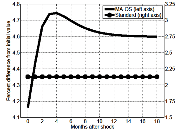
Figure 2: MA-OS Model
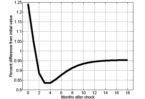
Figure 3: MA-OS Model
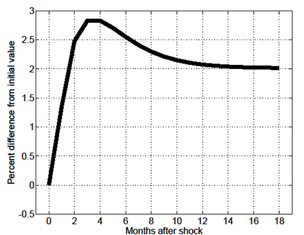
Figure 4: MA-OS Model
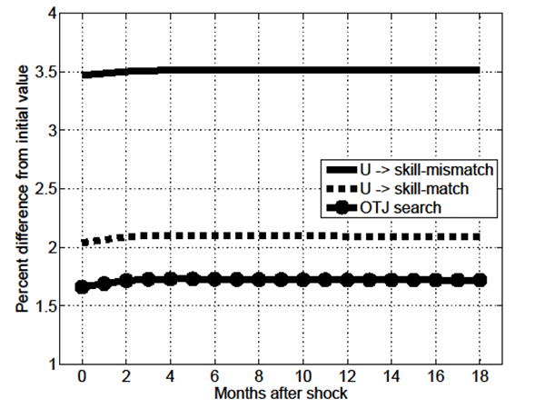
Figure 5: MA-OS Model
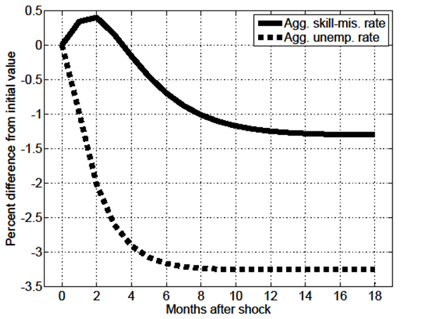
Figure 6: MA-OS Model
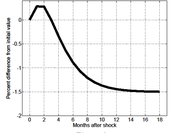
Figures 1-6: responses to 1% permanent (unanticipated)
increase in economy-wide productivity ![]() of V/U ratio
(Fig. 1: MA-OS and Standard models), skill-mismatch probability
of V/U ratio
(Fig. 1: MA-OS and Standard models), skill-mismatch probability
![]() (Fig. 2: MA-OS model),
skill-mismatch to unemployment ratio to
(Fig. 2: MA-OS model),
skill-mismatch to unemployment ratio to ![]() (Fig.
3: MA-OS model), effective search
(Fig.
3: MA-OS model), effective search
![]() : U -
: U - ![]() skill-match,
skill-match,
![]() : U -
: U - ![]() skill-mismatch,
skill-mismatch,
![]() : OTJ search (Fig. 4: MA-OS
model), rate of skill-mismatch
: OTJ search (Fig. 4: MA-OS
model), rate of skill-mismatch ![]() and
unemployment rate
and
unemployment rate ![]() (Fig. 5: MA-OS model), and
fraction of skill-mismatch employment
(Fig. 5: MA-OS model), and
fraction of skill-mismatch employment ![]() (Fig.
6: MA-OS model).
(Fig.
6: MA-OS model).
Figure 7: MA-OS and Standard Models
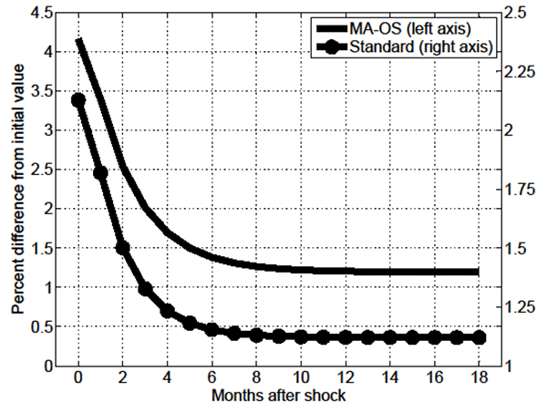
Figure 8: MA-OS and Standard Models
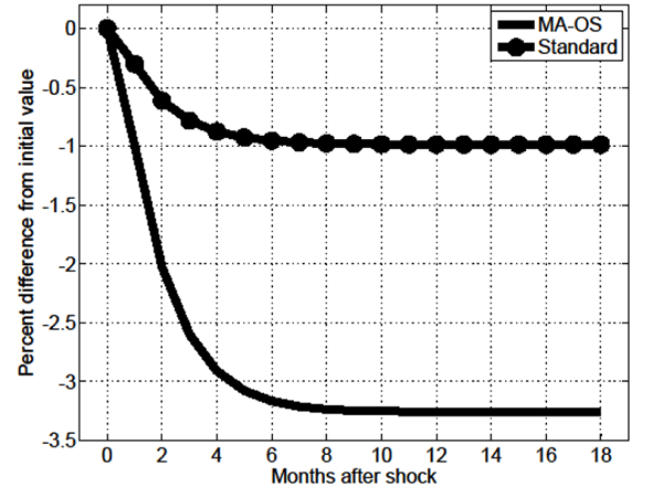
Figure 9: MA-OS and Standard Models
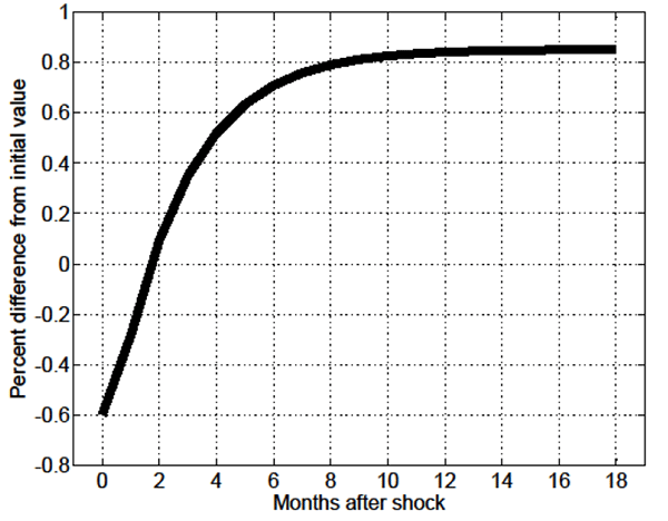
Figure 10: MA-OS and Standard models
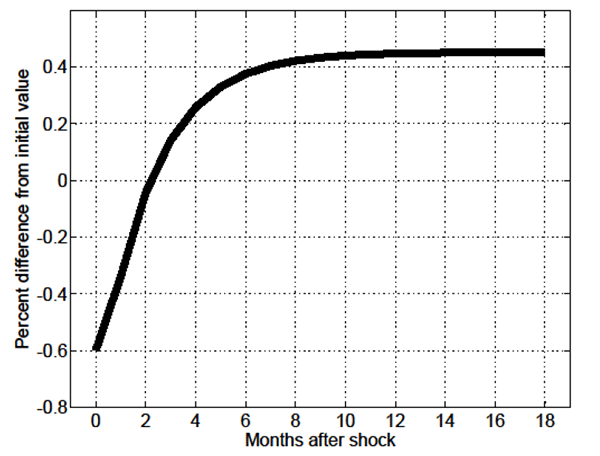
Figure 11: MA-OS and Standard Models
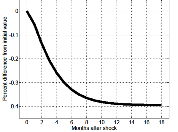
Figure 12: MA-OS and Standard Models
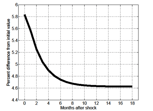
Figures 7-8: responses to 1% permanent (unanticipated)
increase in economy-wide productivity ![]() of aggregate
vacancies
of aggregate
vacancies ![]() (Fig. 7: MA-OS and Standard models)
and aggregate unemployment
(Fig. 7: MA-OS and Standard models)
and aggregate unemployment ![]() (MA-OS and
Standard models).
(MA-OS and
Standard models).
Figures 9-12: responses in MA-OS model to
1% permanent (unanticipated) increase in relative productivity
![]() of V/U ratio (Fig. 9), aggregate
vacancies
of V/U ratio (Fig. 9), aggregate
vacancies ![]() (Fig. 10), aggregate unemployment
(Fig. 10), aggregate unemployment
![]() (Fig. 11), and skill-mismatch probability
(Fig. 11), and skill-mismatch probability
![]() (Fig. 12).
(Fig. 12).
Figure 13: MA-OS and Standard models
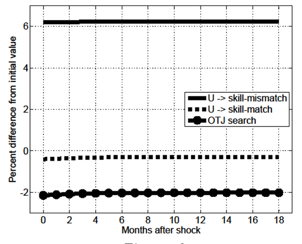
Figure 14: MA-OS and Standard models
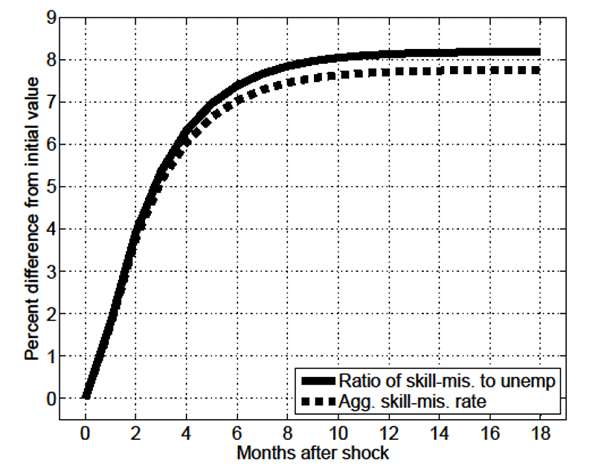
Figure 15: MA-OS and Standard Models
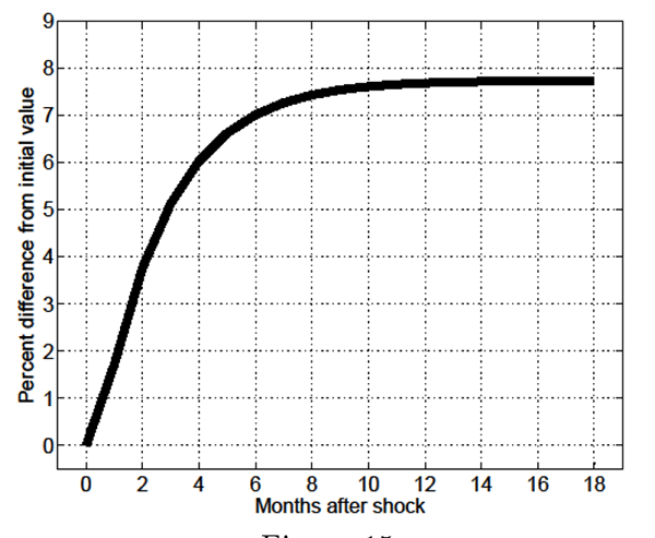
Figure 16: MA-OS and Standard Models
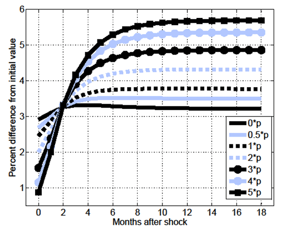
Figure 17: MA-OS and Standard Models
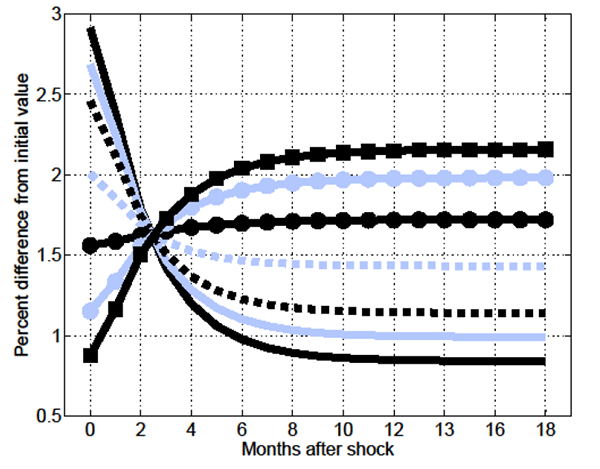
Figure 18: MA-OS and Standard Models
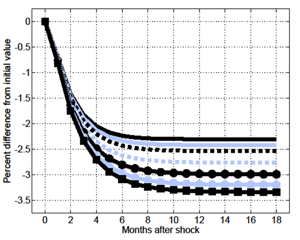
Figures 13-15: responses in MA-OS model to 1% permanent
(unanticipated) increase in relative productivity ![]() of effective search (Fig. 13; legend as in Fig. 4),
rate of skill-mismatch
of effective search (Fig. 13; legend as in Fig. 4),
rate of skill-mismatch ![]() and unemployment rate
(Fig. 14), and fraction of skill-mismatch
employment
and unemployment rate
(Fig. 14), and fraction of skill-mismatch
employment ![]() (Fig. 15).
(Fig. 15).
Figures 16-18
(leg![]() end in Fig. 16 applies to all): responses in MA-OS model
to permanent (unanticipated) increase in economy-wide productivity
end in Fig. 16 applies to all): responses in MA-OS model
to permanent (unanticipated) increase in economy-wide productivity ![]() , and joint shocks in
, and joint shocks in ![]() and relative productivity
and relative productivity ![]() ; 0*p
indicates shock in
; 0*p
indicates shock in ![]() , only. 0.5*p indicates that
size of shock in
, only. 0.5*p indicates that
size of shock in ![]() is half as size as shock to
is half as size as shock to
![]() , etc. In all cases, on impact of exogenous
shocks OPW increases by 0.7%. Response of V/U ratio (Fig. 16),
response of aggregate vacancies
, etc. In all cases, on impact of exogenous
shocks OPW increases by 0.7%. Response of V/U ratio (Fig. 16),
response of aggregate vacancies ![]() (Fig. 17), and
response of aggregate unemployment
(Fig. 17), and
response of aggregate unemployment ![]() (Fig.
18).
(Fig.
18).
Figure 19: MA-OS and Standard Models
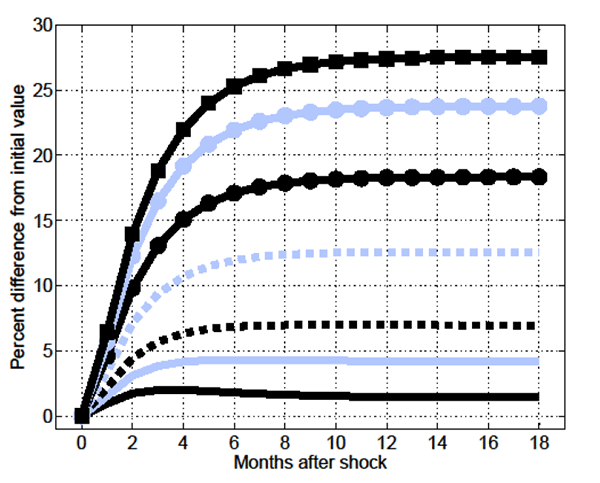
Figure 20: MA-OS and Standard Models
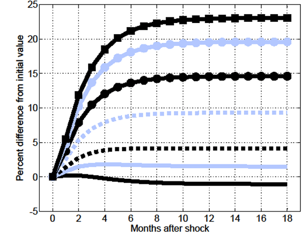
Figures 19-20 (legend in Fig. 16 applies to all):
responses in MA-OS model to permanent (unanticipated) increase in
economy-wide productivity ![]() , and joint shocks
in
, and joint shocks
in ![]() and relative productivity
and relative productivity ![]() ; 0*p indicates shock in
; 0*p indicates shock in ![]() , only. 0.5*p
indicates that size of shock in
, only. 0.5*p
indicates that size of shock in ![]() is half as
size as shock to
is half as
size as shock to ![]() , etc.Response of skill-mismatch to
unemployment ratio
, etc.Response of skill-mismatch to
unemployment ratio ![]() (Fig. 19), and
response of fraction of skill-mismatched employment
(Fig. 19), and
response of fraction of skill-mismatched employment ![]() (Fig. 20).
(Fig. 20).
C Additional Details
As noted in Shimer (2005) and Mortensen and Nagypal (2007), the cyclical properties of models of the sort developed in this paper are well assessed by considering differences between steady states. Therefore, in what follows, relevant mathematical inferences are based on steady-state to steady-state changes.
C.1 The Role of Worker Heterogeneity
Proposition C.1.1. In the
multi-agent model the probability of skill mismatched
employment,
![]() , is countercyclical in
economy-wide productivity
, is countercyclical in
economy-wide productivity ![]() .
.
Proof. Given symmetry, for ![]()
![]() , and
, and
![]() . Then, using
equation
(11) and
rearranging implies that
. Then, using
equation
(11) and
rearranging implies that
![]() ,
where
,
where ![]() , and I have used the assumption that
all effective search is fixed at unity. Therefore, if
, and I have used the assumption that
all effective search is fixed at unity. Therefore, if ![]() is procyclical, then
is procyclical, then
![]() is countercyclical. For
is countercyclical. For
![]() symmetry implies that
symmetry implies that
![]() . Then,
. Then,
 ,
, |
(22) |
since ![]() is procyclical.
is procyclical.
Proposition C.1.2. In the
absence of OTJ search, in the multi-agent model
![]() is (always) constant.
is (always) constant.
Proof. Assuming OTJ search is not possible is equivalent
to setting
![]() , in which case
, in which case
![]() is equal to the constant
is equal to the constant
![]() .
.
Corollary C.1.1. In the
multi-agent model skill-mismatched employment is necessary, but not
sufficient, for propagation in the V/U ratio to occur in response
to changes in economy-wide productivity ![]() .
.
Remark C.1.1. Within the context of the MA-OS model, Proposition 1 can be thought of carrying over as follows: on impact of an increase in economy-wide productivity the probability of skill-mismatch can jump, but relative to its position after this initial jump, the probability of skill-mismatch will thereafter decrease.
The Role of Optimal Effective Search
Proposition C.2.1. In
the standard-OS model effective search is procyclical in
economy-wide productivity ![]() .
.
Proof.25Consistent with the functional forms
assumed for the MA-OS model, for the standard-OS model let
![]() and
and
![]() , where
, where ![]() . In this case,
. In this case,
![]() , where
, where
![]() . Moreover, denote the
job-finding probability of unemployed individuals by
. Moreover, denote the
job-finding probability of unemployed individuals by ![]() , where
, where
![]() . The relevant first-order
condition for optimal search implies that
. The relevant first-order
condition for optimal search implies that
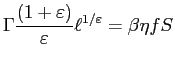 ,
, |
(23) |
where ![]() is the employment surplus (recall that
individuals choose effective search taking market conditions as
given). Moreover, the job-creation condition is now given by
is the employment surplus (recall that
individuals choose effective search taking market conditions as
given). Moreover, the job-creation condition is now given by
| (24) |
Substituting this into equation (23) implies, after total differentiation, that
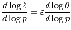 .
. |
(25) |
Since ![]() is procyclical, the equation above
implies that so is effective search
is procyclical, the equation above
implies that so is effective search ![]() . Showing
formally that
. Showing
formally that ![]() is procyclical, to which I now
proceed, offers additional insight. Using the definition of
surplus,
is procyclical, to which I now
proceed, offers additional insight. Using the definition of
surplus, ![]() , and substituting in for the
relevant value functions implies that
, and substituting in for the
relevant value functions implies that
 .
. |
(26) |
Combining with equation (24) yields
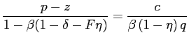 .
. |
(27) |
Therefore,
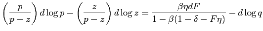 .
. |
(28) |
Using the fact that ![]() and
and
![]() ,
this can be stated as
,
this can be stated as
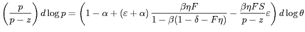 .
. |
(29) |
Of course,
![]() and
and ![]() ,
the latter by assumption: otherwise, it would not be optimal for
individuals to seek employment. Moreover,
,
the latter by assumption: otherwise, it would not be optimal for
individuals to seek employment. Moreover,
![]() ). Then, given
equation
(29), to show
that
). Then, given
equation
(29), to show
that
![]() it is enough to
show that the second term in the coefficient on
it is enough to
show that the second term in the coefficient on
![]() is greater than the third term.
Note that
is greater than the third term.
Note that
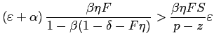
|
|
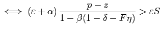
|
|
| (30) |
which will always hold (in the second line above, I have made use
of equation
(26).
Therefore,
![]() ,
,
![]() , and
, and
![]() .
.
Proposition C.2.2. If
effective search is endogenized in the standard model, then the
elasticity of the V/U ratio with respect to economy-wide
productivity ![]() is greater than
otherwise.
is greater than
otherwise.
Proof.26Consistent with the functional forms
assumed for the MA-OS model, for the standard model let
![]() . In this case,
. In this case,
![]() , where
, where
![]() . Moreover, denote the job-finding
probability of unemployed individuals by
. Moreover, denote the job-finding
probability of unemployed individuals by ![]() , where
, where
![]() . Using the definition of
surplus,
. Using the definition of
surplus, ![]() , and substituting in for the
relevant value functions implies that
, and substituting in for the
relevant value functions implies that
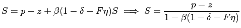 .
. |
(31) |
Combining with the job-creation condition
![]() implies that
implies that
 .
. |
(32) |
Hence,
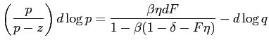 ,
, |
(33) |
and
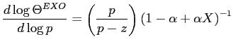 ,
, |
(34) |
Above,
![]() , and
, and
![]() denotes that effective search is
exogenous (and fixed at unity:
denotes that effective search is
exogenous (and fixed at unity: ![]() ). Moreover,
for reasonable values for
). Moreover,
for reasonable values for ![]() ,
, ![]() ,
, ![]() , and
, and ![]() ,
,
![]() .
.
Note from the proof of Proposition 4 that equation (28) can be written as
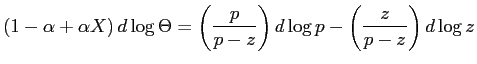
|
|
| |
|
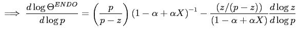
|
|
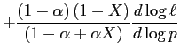 ,
, |
(35) |
where ![]() denotes that effective search is
endogenous. From earlier,
denotes that effective search is
endogenous. From earlier,
![]() ; therefore,
; therefore,
![]() . Moreover, from the
proof of Proposition 4
. Moreover, from the
proof of Proposition 4
![]() and
and
![]() . Of course,
. Of course,
![]() . Hence, using equation
. Hence, using equation
![]() , equation
, equation
![]() can be
stated as
can be
stated as
|
|
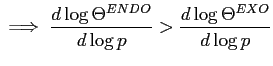 .
. |
(36) |
C.3 Equilibrium in the MA and MA-OS Models
Once searchers ![]() are determined,
sectoral vacancies can be backed out from
are determined,
sectoral vacancies can be backed out from
![]() . Given knowledge of the masses of
unemployed and skill-mismatched individuals it is straightforward
to derive
. Given knowledge of the masses of
unemployed and skill-mismatched individuals it is straightforward
to derive ![]() , and therefore,
, and therefore,
![]() , where
, where ![]() .
Hence, for
.
Hence, for
![]() and
and ![]() knowledge of the key endogenous variables
knowledge of the key endogenous variables
![]() ,
, ![]() ,
,
![]() , and
, and
![]() (eight variables total) is
sufficient to derive all of the model's remaining endogenous
variables. There are four employment values:
(eight variables total) is
sufficient to derive all of the model's remaining endogenous
variables. There are four employment values: ![]() ,
, ![]() ,
, ![]() , and
, and ![]() . Using the
surplus-sharing rule in equation (12) these can be stated in terms of employment surpluses, and solved
for using the four job values implicit in equations (8) and
(9). As
noted before,
. Using the
surplus-sharing rule in equation (12) these can be stated in terms of employment surpluses, and solved
for using the four job values implicit in equations (8) and
(9). As
noted before,
![]() and
and
![]() are defined by the two
corresponding job creation conditions implied by equation (13).
Finally, the remaining six key variables
are defined by the two
corresponding job creation conditions implied by equation (13).
Finally, the remaining six key variables
![]() ,
,
![]() ,
, ![]() ,
,
![]() ,
, ![]() , and
, and
![]() , are defined through the 6
expressions implicit in equations (11), (6), and (7); recall
that the environment is symmetric. Thus, the model reduces to 8
equations in 8 unknowns.
, are defined through the 6
expressions implicit in equations (11), (6), and (7); recall
that the environment is symmetric. Thus, the model reduces to 8
equations in 8 unknowns.
C.4 MA Model: Changes in Relative Productivity
Consider the employment surpluses
and
Given symmetry, for a type-1 firm the expected gains from posting vacancies satisfy
Then, since the skill-mismatch probability is slow moving, what
matters for the on-impact effect of a change in ![]() (or, for that matter, the on-impact effect of a change
in
(or, for that matter, the on-impact effect of a change
in ![]() ), is the expression
), is the expression
From the surplus definitions above, given a change in ![]() , that is, a change that only affects
, that is, a change that only affects ![]() ,
,
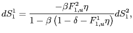
and
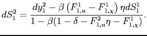
Let
and
Then,
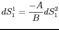 ,
,and
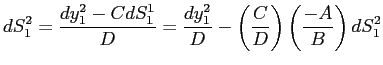
|
|
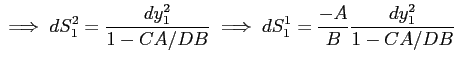 .
. |
Note that if
![]() , then
, then
![]() , meaning that
, meaning that ![]() (for reasonable parameter values, the same is
true when
(for reasonable parameter values, the same is
true when
![]() ), in which
case the sign of
), in which
case the sign of
![]() is equal to the sign of
is equal to the sign of
![]() and the sign of
and the sign of
![]() is opposite to that of
is opposite to that of
![]() . In particular, an increase in
. In particular, an increase in
![]() induces an increase in
induces an increase in ![]() , and therefore an increase in
, and therefore an increase in ![]() and a decrease in
and a decrease in ![]() .
Note, then, that
.
Note, then, that
if and only if
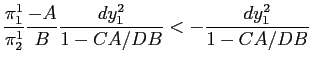 .
.If ![]() this is true if and only if
this is true if and only if

|
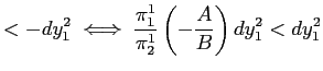
|
|
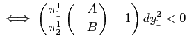 ,
, |
which holds for
![]() since
since ![]() . Therefore, as long as
. Therefore, as long as ![]() ,
an increase in
,
an increase in ![]() induces an on-impact
decrease in the expected gains from posting vacancies.
induces an on-impact
decrease in the expected gains from posting vacancies.
C.5 Matching Function Elasticities
Petrongolo and Pissarides (2001) document that across a wide range of studies aggregate matching functions are found, empirically, to be approximately Cobb-Douglas in aggregate vacancies and unemployment. They note in their concluding section that the coefficient on unemployment is generally found to be in the range 0.5 to 0.7 when matches are formed with individuals exiting unemployment, only, and in the range 0.3-0.4 when total hires are used as the dependent variable (not only hires from unemployment). The nature of the standard and standard-OS models is such that the former applies, while the latter applies to the MA and MA-OS models.
In the standard and standard-OS models total matches are given
by
![]() , where
, where
![]() denotes effective search; it clearly
follows that in both cases the partial elasticities of
denotes effective search; it clearly
follows that in both cases the partial elasticities of ![]() with respect to
with respect to ![]() and
and ![]() are,
respectively,
are,
respectively, ![]() and
and ![]() . In
the MA and MA-OS models, given sectoral matching functions and
symmetry, it is straightforward to show that total matches in the
economy are given by
. In
the MA and MA-OS models, given sectoral matching functions and
symmetry, it is straightforward to show that total matches in the
economy are given by
where
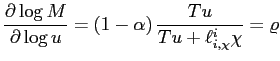 .
.As the effective fraction of on-the-job searchers converges to
zero, this elasticity converges to
![]() ,
,
as in the standard
model. As long as
![]() and
and
![]() , then
, then
![]() . Furthermore,
. Furthermore,
![]() if and only if
if and only if
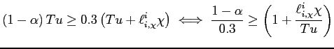 .
.Numerical analysis reveals that
![]() . Hence, for
. Hence, for
![]() , the partial elasticities of
aggregate matches with respect to
, the partial elasticities of
aggregate matches with respect to ![]() and
and
![]() are broadly consistent with the findings
in Petrongolo and Pissarides (2001).
are broadly consistent with the findings
in Petrongolo and Pissarides (2001).
C.6 Sensitivity to Changes in Key Parameters/Variables
Table C.6.1 Model calibrations (weekly frequency)
| Difference in | Parameter: b | Parameter: ∝ | Parameter: A | Parameter: T | Parameter: c | Parameter: Ø | Parameter: ε | Parameter: δ | Parameter: ß | Parameter: η |
|---|---|---|---|---|---|---|---|---|---|---|
| none | 0.72 | 0.60 | 0.20 | 1.00 | 0.72 | 0.12 | 1.00 | 0.0081 | 0.999 | 0.50 |
| ε | 0.73 | 0.60 | 0.20 | 1.00 | 0.70 | 0.12 | 1.10 | 0.0081 | 0.999 | 0.50 |
| Ø | 0.72 | 0.60 | 0.20 | 1.00 | 0.71 | 0.13 | 1.00 | 0.0081 | 0.999 | 0.50 |
| η | 0.72 | 0.60 | 0.19 | 1.00 | 0.60 | 0.12 | 1.00 | 0.0081 | 0.999 | 0.55 |
| z | 0.75 | 0.60 | 0.20 | 1.00 | 0.63 | 0.13 | 1.00 | 0.0081 | 0.999 | 0.50 |
Notes for reference, first row shows benchmark
calibration; second row refers to calibration in which
![]() is 10 percent higher, but all
targets remain as in benchmark; third row refers to calibration in
which
is 10 percent higher, but all
targets remain as in benchmark; third row refers to calibration in
which ![]() is 10% higher, but all targets remain
as in benchmark except that implied ratio of skill-mismatched wage
to average sectoral wage is now 0.83; fourth row refers to
calibration in which
is 10% higher, but all targets remain
as in benchmark except that implied ratio of skill-mismatched wage
to average sectoral wage is now 0.83; fourth row refers to
calibration in which ![]() is 10% higher, but all
targets remain as in benchmark; fifth row refers to case in which
net unemployment flow benefits
is 10% higher, but all
targets remain as in benchmark; fifth row refers to case in which
net unemployment flow benefits ![]() are targeted to be
10% higher (0.55 instead of 0.5), but all other targets remain as
in benchmark.
are targeted to be
10% higher (0.55 instead of 0.5), but all other targets remain as
in benchmark.
Table C.6.2: properties of key variables under ε = 1:1
| V/U Ratio: C1 | V/U Ratio: C2 | V/U Ratio: C3 | Vacancies: C4 | Vacancies: C5 | Vacancies: C6 | Unemp.: C7 | Unemp.: C8 | ∂v/∂u C9 | OPW: C10 | |
|---|---|---|---|---|---|---|---|---|---|---|
| R1: US | 7.79 | 12 | 60% | 3.88 | 12 | 60% | -3.93 | 15 | -0.86 | - |
| R2: MA-OS | 4.81 | 4 | 11% | 1.22 | 0 | 0% | -3.47 | 11 | -0.35 | 1.00 |
| R3: MA-OS | 5.22 | 7 | 22% | 1.43 | 0 | 0% | -3.65 | 12 | -0.39 | 0.99 |
| R4: MA-OS | 5.66 | 8 | 32% | 1.68 | 0 | 0% | -3.83 | 12 | -0.44 | 0.99 |
| R5: MA-OS | 6.52 | 15 | 50% | 2.15 | 0 | 0% | -4.19 | 12 | -0.51 | 0.97 |
| R6: MA-OS | 7.40 | 15 | 63% | 2.62 | 0 | 0% | -4.55 | 13 | -0.58 | 0.96 |
| R7: MA-OS | 8.22 | 16 | 73% | 3.10 | 12 | 26% | -4.89 | 13 | -0.63 | 0.95 |
| R8: MA-OS | 8.79 | 16 | 78% | 3.37 | 13 | 43% | -5.12 | 14 | -0.66 | 0.94 |
Notes: Alternative calibration that applies to results in
![]() -
-![]() implements value
for
implements value
for
![]() 10% higher than in benchmark
calibration, but all targets remain the same.
10% higher than in benchmark
calibration, but all targets remain the same. ![]() : elasticity of V/U ratio with respect to output per worker
(OPW);
: elasticity of V/U ratio with respect to output per worker
(OPW); ![]() : months after shock over which V/U ratio
continues to increase (propagation);
: months after shock over which V/U ratio
continues to increase (propagation); ![]() : percent of
total increase in V/U ratio occurring over period of slow-moving
adjustment;
: percent of
total increase in V/U ratio occurring over period of slow-moving
adjustment; ![]() : elasticity of aggregate vacancies
with respect to OPW;
: elasticity of aggregate vacancies
with respect to OPW; ![]() : months after shock over
which vacancies continue to increase (propagation);
: months after shock over
which vacancies continue to increase (propagation); ![]() : percent of total increase in vacancies occurring over
period of slow-moving adjustment;
: percent of total increase in vacancies occurring over
period of slow-moving adjustment; ![]() : elasticity
of aggregate unemployment with respect to OPW;
: elasticity
of aggregate unemployment with respect to OPW; ![]() : month at which unemployment reaches a trough;
: month at which unemployment reaches a trough; ![]() : slope of Beveridge curve;
: slope of Beveridge curve; ![]() :
elasticity of output per worker with respect to on-impact size of
exogenous shock (0.007).
:
elasticity of output per worker with respect to on-impact size of
exogenous shock (0.007). ![]() : US data;
: US data; ![]() : responses given
: responses given ![]() -induced on-impact
increase in OPW of 0.7% under benchmark calibration;
-induced on-impact
increase in OPW of 0.7% under benchmark calibration; ![]() -
-![]() : response in MA-OS model to joint
increases in
: response in MA-OS model to joint
increases in ![]() and
and ![]() that (in all
cases) induce an on-impact increase in OPW of 0.7%, where size of
shock to
that (in all
cases) induce an on-impact increase in OPW of 0.7%, where size of
shock to ![]() is half of shock in
is half of shock in ![]() (
(![]() ), equal to shock in
), equal to shock in ![]() (
(![]() ), and two (
), and two (![]() ), three
(
), three
(![]() ), four (
), four (![]() ), and five
(
), and five
(![]() ) times the shock in
) times the shock in ![]() .
.
Table C.6.3: properties of key variables under φ = 0:13
| V/U Ratio: C1 | V/U Ratio: C2 | V/U Ratio: C3 | Vacancies: C4 | Vacancies: C5 | Vacancies: C6 | Unemp.: C7 | Unemp.: C8 | ∂v/∂u C9 | OPW: C10 | |
|---|---|---|---|---|---|---|---|---|---|---|
| R 1: US | 7.79 | 12 | 60% | 3.88 | 12 | 60% | -3.93 | 15 | -0.86 | - |
| R2: MA-OS | 4.62 | 4 | 12% | 1.22 | 0 | 0% | -3.29 | 10 | -0.37 | 1.00 |
| R3: MA-OS | 5.03 | 5 | 23% | 1.43 | 0 | 0% | -3.47 | 10 | -0.41 | 1.00 |
| R4: MA-OS | 5.45 | 9 | 34% | 1.65 | 0 | 0% | -3.66 | 11 | -0.45 | 0.99 |
| R5: MA-OS | 6.30 | 11 | 52% | 2.10 | 0 | 0% | -4.03 | 11 | -0.52 | 0.98 |
| R6: MA-OS | 7.15 | 14 | 65% | 2.54 | 6 | 2% | -4.40 | 13 | -0.58 | 0.96 |
| R7: MA-OS | 7.94 | 15 | 76% | 2.95 | 11 | 34% | -4.75 | 14 | -0.62 | 0.95 |
| R8: MA-OS | 8.49 | 15 | 81% | 3.22 | 12 | 51% | -4.98 | 15 | -0.65 | 0.95 |
Notes: Alternative calibration that applies to results in
![]() -
-![]() implements
skill-mismatch parameter 10% higher than in benchmark calibration,
but all targets remain the same. Row and column references are as
in Table C.5.2.
implements
skill-mismatch parameter 10% higher than in benchmark calibration,
but all targets remain the same. Row and column references are as
in Table C.5.2.
Table C.6.4: properties of key variables under η = 0:55
| V/U Ratio: C1 | V/U Ratio: C2 | V/U Ratio: C3 | Vacancies: C4 | Vacancies: C5 | Vacancies: C6 | Unemp.: C7 | Unemp.: C8 | ∂v/∂u C9 | OPW: C10 | |
|---|---|---|---|---|---|---|---|---|---|---|
| R 1: US | 7.79 | 12 | 60% | 3.88 | 12 | 60% | -3.93 | 15 | -0.86 | - |
| R2: MA-OS | 4.61 | 4 | 14% | 1.21 | 0 | 0% | -3.28 | 9 | -0.37 | 1.00 |
| R3: MA-OS | 5.06 | 6 | 26% | 1.45 | 0 | 0% | -3.48 | 12 | -0.42 | 1.00 |
| R4: MA-OS | 5.52 | 9 | 37% | 1.67 | 0 | 0% | -3.69 | 11 | -0.46 | 0.99 |
| R5: MA-OS | 6.43 | 12 | 56% | 2.16 | 0 | 0% | -4.09 | 12 | -0.53 | 0.98 |
| R6: MA-OS | 7.35 | 14 | 70% | 2.63 | 13 | 17% | -4.50 | 13 | -0.59 | 0.96 |
| R7: MA-OS | 8.20 | 15 | 81% | 3.07 | 13 | 49% | -4.87 | 13 | -0.63 | 0.96 |
| R8: MA-OS | 8.79 | 18 | 87% | 3.36 | 18 | 66% | -5.12 | 14 | -0.66 | 0.95 |
Notes: Alternative calibration that applies to results in
![]() -
-![]() implements
bargaining power of workers 10% higher than in benchmark
calibration, but all targets remain the same. Row and column
references are as in Table C.5.2.
implements
bargaining power of workers 10% higher than in benchmark
calibration, but all targets remain the same. Row and column
references are as in Table C.5.2.
Table C.6.5: properties of key variables under z = 0:55
| V/U Ratio: C1 | V/U Ratio: C2 | V/U Ratio: C3 | Vacancies: C4 | Vacancies: C5 | Vacancies: C6 | Unemp.: C7 | Unemp.: C8 | ∂v/∂u C9 | OPW: C10 | |
|---|---|---|---|---|---|---|---|---|---|---|
| R 1: US | 7.79 | 12 | 60% | 3.88 | 12 | 60% | -3.93 | 15 | -0.86 | - |
| R2: MA-OS | 5.19 | 4 | 13% | 1.38 | 0 | 0% | -3.67 | 9 | -0.38 | 1.00 |
| R3: MA-OS | 5.65 | 6 | 24% | 1.62 | 0 | 0% | -3.88 | 10 | -0.42 | 1.00 |
| R4: MA-OS | 6.12 | 8 | 34% | 1.87 | 0 | 0% | -4.10 | 11 | -0.46 | 0.99 |
| R5: MA-OS | 7.06 | 12 | 50% | 2.36 | 0 | 0% | -4.48 | 14 | -0.53 | 0.97 |
| R6: MA-OS | 8.00 | 13 | 63% | 2.86 | 0 | 0% | -4.89 | 15 | -0.59 | 0.96 |
| R7: MA-OS | 8.90 | 13 | 73% | 3.32 | 10 | 27% | -5.27 | 15 | -0.63 | 0.95 |
| R8: MA-OS | 9.51 | 15 | 78% | 3.64 | 12 | 43% | -5.53 | 16 | -0.66 | 0.94 |
Notes: Alternative calibration that applies to results in
![]() -
-![]() targets net
unemployment flow benefits 10% higher than in benchmark
calibration, while all other targets remain the same. Row and
column references are as in Table C.5.2.
targets net
unemployment flow benefits 10% higher than in benchmark
calibration, while all other targets remain the same. Row and
column references are as in Table C.5.2.
Footnotes
**. International Finance Division, Board of Governors of the Federal Reserve System, Washington, D.C. 20551. E-mail: [email protected]. My greatest thanks to Mike Elsby, Etienne Gagnon, Miles Kimball, Toshihiko Mukoyama, Jeff Smith, and Brian Jacob for very helpful comments and discussions, and also to seminar participants at the Board of Governors of the Federal Reserve System, Brown University, McMaster University, the University of Michigan, the 2012 Midwest Macro Meetings hosted by the University of Notre Dame, and the 2012 Canadian Economics Association annual conference hosted by the University of Calgary. All errors are my own. The views in this paper are solely the responsibility of the author and should not be interpreted as reflecting the views of the Board of Governors of the Federal Reserve System or of any other person associated with the Federal Reserve System. Return to text
1. See, for example, Shimer (2005), Hall (2005), Fujita and Ramey (2007), Mortensen and Nagypal (2007), and Hagedorn and Manovskii (2008) for additional discussion on the V/U ratio's emprical response to changes in productivity, and also with regards to the standard/benchmark model's limitations in fully accounting for the data. In broader reference to the standard model, see, for instance Diamond (1982), Pissarides (1985), Mortensen and Pissarides (1994), and Pissarides (2000). Return to text
2. In particular, given an increase in productivity of about 0.7% the V/U ratio jumps and thereafter continues to slowly rise over approximately 12 months. Return to text
3. As is standard in the literature, by this I mean an exogenous change in productivity. Return to text
4. I assume that it is always optimal for them to do so, as the central focus of this paper is tied to examining the implications of skill-mismatched employment. Return to text
5. I elaborate on the meaning of surplus further below, as well as on the overall determination of wages. Return to text
6. This is based on the theory developed in Pissarides (2000), chapter 5, in which the standard, homogeneous-agent model features an endogenous job-seeking technological component. Later in the paper I endogenize the choice of idiosyncratic search technologies within the present multi-agent framework. Return to text
7. Total matches in sector-1 are given by
8. See the appendix for further details Return to text
9. See, for instance, Pissarides (2000). Return to text
10. See the appendix for further details. Return to text
11. Indeed, numerical analysis implies
that
![]() is
endogenously optimal. Quite simply, this captures differences in
outside options between unemployed and OTJ searchers. Return to text
is
endogenously optimal. Quite simply, this captures differences in
outside options between unemployed and OTJ searchers. Return to text
12. In their cross-country investigation, Krueger and Mueller (2008) find that, conditional on searching, the average search time ranges from 40 minutes per week in Slovenia, to slightly less than 4 hours per week in Canada (which is a small amount more than in the U.S.). Return to text
13. Individuals choose effective search
taking market conditions as given (in particular,
![]() ). Note that it is endogenously
optimal to set
). Note that it is endogenously
optimal to set
![]() . Return to text
. Return to text
14. See the appendix, as well as Pissarides (2000), chapter 5, for further details on what I refer to as the "standard-OS model." Return to text
15. With regards to procyclical effective search, see, for instance, Christensen et al. (2005). As noted earlier, the procyclicality of effective search is also a feature of the standard, homogenous-agent model enhanced to account for endogenous effective search (Pissarides (2000), chapter 5). Return to text
16. Numerical analysis reveals that differences in results stemming from temporary and permanent changes in the economy's driving forces are for all purposes negligible. In terms of impulse response functions, in particular, differences are broadly limited to the absence of mean reversion. This is broadly in line with the fact that, as noted in Shimer (2005) and Mortensen and Nagypal (2007), the cyclical properties of models of the sort developed in the present paper are well assessed by considering differences between steady states. Return to text
17. The unemployment rate ![]() is at monthly frequency, spans 1951:M1 through 2011:M10, and is
taken from the Bureau of Labor Statistics (BLS). Vacancies
is at monthly frequency, spans 1951:M1 through 2011:M10, and is
taken from the Bureau of Labor Statistics (BLS). Vacancies
![]() are at monthly frequency and obtained by
using the Job Openings and Labor Turnover Survey (JOLTS) data since
2000:M12 (when first available) combined with the Conference
Board's Help-Wanted Index (HWI) from 1951:M1 through 2000:M11
(adjusted to the JOLTS units of measurement). Return to text
are at monthly frequency and obtained by
using the Job Openings and Labor Turnover Survey (JOLTS) data since
2000:M12 (when first available) combined with the Conference
Board's Help-Wanted Index (HWI) from 1951:M1 through 2000:M11
(adjusted to the JOLTS units of measurement). Return to text
18. See the appendix for further details. Return to text
19. The appendix shows that implementing
alternative values for ![]() ,
,
![]() ,
, ![]() and
and
![]() does not substantially alter overall
results. Return to text
does not substantially alter overall
results. Return to text
20. To further understand this, consider
an extreme example. Suppose the expected gains from
skill-mismatched search were zero; then, the first-order conditions
for optimal effective search imply that
![]() would be zero as well. Given
a positive productivity shock, assume these expected gains increase
by an arbitrarily small amount. Then, so will
would be zero as well. Given
a positive productivity shock, assume these expected gains increase
by an arbitrarily small amount. Then, so will
![]() . However, because
. However, because
![]() was originally zero, the
percent change in
was originally zero, the
percent change in
![]() would technically be
infinity. However, recall from earlier that by comparative
advantage
would technically be
infinity. However, recall from earlier that by comparative
advantage
![]() in all
states of the economy. Return to
text
in all
states of the economy. Return to
text
21. See, for instance, Pissarides (2009). Return to text
22. Empirical elasticities are based off
the logarithm of quarterly data spanning 1951:Q1 through 2011:Q3
that, following Shimer (2005), is detrended using an HP-filter with
smoothing parameter ![]() . Data on unemployment
and output per worker is taken from Bureau of Labor Statistics.
Vacancies are obtained by using the Job Openings and Labor Turnover
Survey (JOLTS) data since 2000:M12 (when first available) combined
with the Conference Board's Help-Wanted Index (HWI) from 1951:M1
through 2000:M11 (adjusted to the JOLTS units of measurement). Both
unemployment and vacancy data are originally at monthly frequency
(statistics are based off quarterly averages); the series of output
per worker is only available at quarterly frequency. Return to text
. Data on unemployment
and output per worker is taken from Bureau of Labor Statistics.
Vacancies are obtained by using the Job Openings and Labor Turnover
Survey (JOLTS) data since 2000:M12 (when first available) combined
with the Conference Board's Help-Wanted Index (HWI) from 1951:M1
through 2000:M11 (adjusted to the JOLTS units of measurement). Both
unemployment and vacancy data are originally at monthly frequency
(statistics are based off quarterly averages); the series of output
per worker is only available at quarterly frequency. Return to text
23. In line with the overall preceding analysis, note that in all cases referred to henceforth, model-generated elasticities are based off permanent changes in productivity, and hence are implied by changes between steady states. Return to text
24. In particular, net unemployment flow
benefits must be approximately 96% of OPW in order for the standard
model to match the data's amplification properties. Recall that the
present calibration is such that net unemployment flow benefits are
approximately 50% of OPW. Intuitively, the fact that employment
surpluses are a function of the difference between the productivity
of a match and net unemployment flow benefits means that the
smaller this difference is, the more percentage-wise sensitive it
is to changes in productivity, and therefore, the greater the
elasticity of ![]() with respect to
OPW. Return to text
with respect to
OPW. Return to text
25. For simplicity, this proof assumes functional forms consistent with the overall development of the model. Return to text
26. For simplicity, this proof assumes functional forms consistent with the overall development of the model. Return to text
This version is optimized for use by screen readers. Descriptions for all mathematical expressions are provided in LaTex format. A printable pdf version is available. Return to text