Skip to: [Printable Version (PDF)]

Board of Governors of the Federal Reserve System
International Finance Discussion Papers
Number 1063, November 2012 --- Screen Reader Version*

Fiscal Consolidation in a Currency Union: Spending Cuts vs. Tax Hikes¹

Christopher J. Erceg and Jesper Lindé²

NOTE: International Finance Discussion Papers are preliminary materials circulated to stimulate discussion and critical comment. References in publications to International Finance Discussion Papers (other than an acknowledgment that the writer has had access to unpublished material) should be cleared with the author or authors. Recent IFDPs are available on the Web at http://www.federalreserve.gov/pubs/ifdp/. This paper can be downloaded without charge from the Social Science Research Network electronic library at http://www.ssrn.com/.

Abstract:

This paper uses a two country DSGE model to examine the effects of tax-based versus expenditure-based fiscal consolidation in a currency union. We find three key results. First, given limited scope for monetary accommodation, tax-based consolidation tends to have smaller adverse effects on output than expenditure-based consolidation in the near-term, though is more costly in the longer-run. Second, a large expenditure-based consolidation may be counterproductive in the near-term if the zero lower bound is binding, reflecting that output losses rise at the margin. Third, a "mixed strategy" that combines a sharp but temporary rise in taxes with gradual spending cuts may be desirable in minimizing the output costs of fiscal consolidation.

Keywords: Monetary policy, fiscal policy, liquidity trap, zero bound constraint, open economy macroeconomics, DSGE model

JEL classification: E32, F41

1.  Introduction

The global financial crisis and slow ensuing recovery have put severe strains on the fiscal positions of many industrial countries. Between 2007 and 2011, debt/GDP ratios climbed by 25 to 30 percent in many countries, including the United States, United Kingdom, France, and Spain. Mounting concern about high and rising debt levels, especially in the wake of the runup in borrowing costs for many European sovereigns, has spurred efforts to implement sizeable and long-lived fiscal consolidation plans, especially in Europe.

In designing a fiscal consolidation plan, policymakers must make a number of key decisions: These include the size of the desired improvement in the primary balance or debt/GDP ratio; its composition between spending cuts and tax increases; and its speed of implementation. Thus far, many of the fiscal consolidation plans in Europe that have received legislative approval appear to have broadly similar features - they are typically fairly front-loaded, and more focused on spending cuts than tax-hikes. But an important open question is the extent to which it may be desirable to tailor the structure of fiscal consolidation to the economy in question by taking account of its monetary policy regime, the state of the business cycle, and other factors.

Our paper makes a purely positive contribution along these lines by investigating how the effects of tax-based versus expenditure-based consolidation depend on the degree of monetary accommodation.³ Specifically, we use a two country medium-sized DSGE model to analyze the implications of each type of consolidation under the constraints imposed by currency union membership. We consider an independent monetary policy (IMP) as a useful reference point, and allow for the possibility that the currency union is constrained by the ZLB. Our analysis has an important parallel with previous work by Eggertsson (2010), who used the New Keynesian model to compare the relative efficacy of spending hikes and tax cuts in providing short-run fiscal stimulus when the ZLB is binding. However, our analysis differs due to its open economy orientation, our use of a more empirically-realistic model, and our focus on longer-term fiscal consolidation.

Our model assumes that the home economy is large enough to markedly influence the setting of policy rates, so that fiscal consolidation may affect the duration of the liquidity trap faced by the currency union. Fiscal policy in each country specifies a rule for how either the labor tax rate or government spending responds to the difference between the debt/GDP ratio and its target value, with the latter time-varying. An important feature influencing the effects of fiscal policy in our model is the inclusion of "rule of thumb" households who consume all of their after-tax income as in Erceg, Guerrieri, and Gust (2006); ample micro- and macro-evidence suggests that such non-Ricardian consumption behavior is a key transmission channel for fiscal policy.⁴ On other dimensions, our model is a relatively standard two country open economy model which embeds the nominal and real frictions that have been identified as empirically important in the closed economy models of Christiano, Eichenbaum, and Evans (2005) and Smets and Wouters (2003), as well as analogous frictions relevant in an open economy framework (such as costs of adjusting trade flows). Given the importance of financial frictions as an amplification mechanism - as highlighted by the recent work of Christiano, Motto and Rostagno (2010) - we incorporate a financial sector following the basic approach of Bernanke, Gertler, and Gilchrist (1999).

We begin by analyzing the effects of a 25 percent reduction in the desired long-run debt target that is achieved either by a prolonged rise in the labor tax rate, or alternatively, through a cut in government spending. Under an independent monetary policy (IMP), government spending cuts are much less costly in reducing public debt than tax hikes. With a tax hike, output falls 2 percent after two years, while the debt/GDP ratio is reduced about 4 percentage points, consistent with a "fiscal sacrifice ratio" of 1/2 at a two year horizon. By contrast, output falls only about half as much under the spending-based consolidation, while progress in reducing debt is slightly faster, implying a sacrifice ratio of less than 1/4. The larger output decline in response to tax hikes reflects that tax hikes have a more depressing effect on potential output, and that monetary policy (which follows a Taylor rule) keeps output reasonably close to potential under either type of consolidation.⁵ A key insight is that the spending-based consolidation requires relatively large cuts in the policy rate to crowd-in private demand, including through an induced depreciation of the exchange rate, while the tax-based consolidation implies a much smaller fall in interest rates, and generates exchange rate appreciation.

Under a currency union, an expenditure-based consolidation depresses output by more than a tax-based consolidation for several years. This reflects that the CU central bank in effect provides too little accommodation given its focus on union-wide aggregates. Moreover, fixed exchange rates tend to cause spending cuts to be more contractionary than under an IMP, while causing tax hikes to be somewhat less contractionary (by reducing the appreciation that would otherwise occur). Even so, because real interest rates and real exchange rates gradually adjust towards their flexible price levels at longer horizons, the sacrifice ratio associated with a spending-based consolidation eventually falls below that of a tax-based consolidation, with the cross-over occurring after three years under our benchmark calibration. Thus, the CU constraint in effect introduces an intertemporal trade-off between tax-based and expenditure-based consolidation: the former induces a smaller near-term output contraction, but implies a considerably deeper output decline at longer horizons.

The adverse GDP impact of a spending-based consolidation is exacerbated considerably when the CU central bank is constrained by the ZLB. Given the substantial size of the home country in the CU, larger spending cuts lengthen the duration of the liquidity trap faced by the CU, implying a progressively larger adverse impact on output at the margin (i.e., the multiplier increases), and correspondingly, less improvement in the debt/GDP. If large enough in scale, spending-based consolidations can even become counterproductive at a horizon extending out several years, in the sense that they markedly deepen the output contraction without achieving any additional improvement in the debt/GDP ratio. By contrast, the effects of tax-based consolidation are much less sensitive to the degree of monetary accommodation, and hence to the scale of fiscal consolidation: the sacrifice ratio is close to constant until the consolidation becomes extremely large.

Given that tax-based consolidations are relatively attractive in the near-term if monetary policy is constrained, while spending-based consolidations induce a smaller longer-term output contraction, it is natural to consider the effects of a "mixed strategy" that combines sharp but temporary increases in taxes with more gradual and more persistent spending cuts. We find that such an approach indeed contributes to much smaller output costs in the near-term than under a spending-based approach, while also reducing the longer-run output contraction (since taxes are lower in the longer-term). Of course, the benign effects on output are contingent on convincing the public that the tax hikes are purely temporary, which may be difficult to achieve in practice given that tax hikes initially promised as temporary often prove hard to unwind. If the public believes the tax hike will ultimately support higher spending, the effects on output would be much more contractionary.

We also illustrate how the model's implications for sacrifice ratio under alternative types of consolidation are sensitive to a number of key parameters. Perhaps unsurprisingly, a high Frisch elasticity of labor supply tends to make spending-based consolidation more attractive at all horizons. The sharp contractionary effects of spending-based consolidations are mitigated with a flatter Phillips Curve slope; even so, tax-based consolidations continue to imply a smaller output contraction for several years and generate a faster debt improvement under an extremely flat Phillips Curve.

Overall, our results clearly underscore the importance of structuring fiscal consolidation to take account of constraints on interest rate and exchange rate adjustment. Our analysis can be regarded as merging insights from several strands of the literature. In the spirit of Eggertsson (2010), we find that constraints on monetary accommodation - in our case, extended to an open economy setting - can make tax hikes appear relatively more attractive than spending cuts in achieving fiscal consolidation.⁶ Even so, consistent with the implications of "textbook" Keynesian models and the VAR-based analysis of Blanchard and Perotti (2002) - but not with Eggertsson's stylized New Keynesian model - we find that both tax hikes and spending cuts are contractionary in all of the monetary environments we consider.⁷ Finally, the implication that spending-based consolidation has much less costly effects on output than tax-based consolidation in the longer-term is consistent with the supply-side effects emphasized in Uhlig (2010).

The reminder of the paper is organized as follows. Section 2 presents our workhorse two country model, and Section 3 discusses the calibration and solution procedure. The results for the benchmark calibration are reported in Section 4, while Section 5 assesses sensitivity to alternative parameterizations. Section 6 concludes.

2.  The Model

Our modeling framework is very similar to Erceg and Lindé (2010a) aside from some features of the fiscal policy specification. Our model consists of two countries (or country blocks) that differ in size, but are otherwise isomorphic. The first country is the home economy, or "South", while the second country is referred to as the "North." The countries share a common currency, and monetary policy is conducted by a single central bank. During "normal" times when the zero bound constraint on policy rates is not binding, the central bank adjusts policy rates in response to the aggregate inflation rate and output gap of the currency union. By contrast, fiscal policy may differ across the two blocks. Given the isomorphic structure, our exposition below largely focuses on the structure of the South.

As the recent recession has provided strong evidence in favor of the importance of financial frictions, our model also features a financial accelerator channel which closely parallels earlier work by Bernanke, Gertler, and Gilchrist (1999) and Christiano, Motto, and Rostagno (2008). Given that the mechanics underlying this particular financial accelerator mechanism are well-understood, we simplify our exposition by focusing on a special case of our model which abstracts from a financial accelerator. We conclude our model description with a brief description of how the model is modified to include the financial accelerator (Section 2.6).

2.1  Firms and Price Setting

2.1.1  Production of Domestic Intermediate Goods

There is a continuum of differentiated intermediate goods (indexed by $i\in\lbrack0,1]$) in the South, each of which is produced by a single monopolistically competitive firm. In the domestic market, firm $i$ faces a demand function that varies inversely with its output price $P_{Dt}(i)$ and directly with aggregate demand at home $Y_{Dt}$:

$$Y_{Dt}(i)=\left[ \frac{P_{Dt}(i)}{P_{Dt}}\right] ^{\frac{-\left( 1+\theta_{p}\right) }{\theta_{p}}}Y_{Dt},$$ (1)

where $\theta_{p}>0$, and $P_{Dt}$ is an aggregate price index defined below. Similarly, firm $i$ faces the following export demand function:

$$X_{t}(i)=\left[ \frac{P_{Mt}^{\ast}(i)}{P_{Mt}^{\ast}}\right] ^{\frac {-\left( 1+\theta_{p}\right) }{\theta_{p}}}M_{t}^{\ast} ,$$ (2)

where $X_{t}(i)$ denotes the quantity demanded of domestic good $i$ in the North block, $P_{Mt}^{\ast}(i)$ denotes the price that firm $i$ sets in the North market, $P_{Mt}^{\ast}$ is the import price index in the North, and $M_{t}^{\ast}$ is an aggregate of the North's imports (we use an asterisk to denote the North's variables).

Each producer utilizes capital services $K_{t}\left( i\right)$ and a labor index $L_{t}\left( i\right)$ (defined below) to produce its respective output good. The production function is assumed to have a constant-elasticity of substitution (CES) form:

$$Y_{t}\left( i\right) =\left( \omega_{K}^{\frac{\rho}{1+\rho}} K_{t}(i)^{\frac{1}{1+\rho}}+\omega_{L}{}^{\frac{\rho}{1+\rho}}(Z_{t} L_{t}(i))^{\frac{1}{1+\rho}}\right) ^{1+\rho}.$$ (3)

The production function exhibits constant-returns-to-scale in both inputs, and $Z_{t}$ is a country-specific shock to the level of technology. Firms face perfectly competitive factor markets for hiring capital and labor. Thus, each firm chooses $K_{t}\left( i\right)$ and $L_{t}\left( i\right)$, taking as given both the rental price of capital $R_{Kt}$ and the aggregate wage index $W_{t}$ (defined below). Firms can costlessly adjust either factor of production, which implies that each firm has an identical marginal cost per unit of output, $MC_{t}$. The (log-linearized) technology shock is assumed to follow an AR(1) process:

$$z_{t}=\rho_{z}z_{t-1}+\varepsilon_{z,t}.$$ (4)

We assume that purchasing power parity holds, so that each intermediate goods producer sets the same price $P_{Dt}(i)$ in both blocks of the currency union, implying that $P_{Mt}^{\ast}(i)=P_{Dt}(i)$ and that $P_{Mt}^{\ast}=P_{Dt}$. The prices of the intermediate goods are determined by Calvo-Yun style staggered contracts (see Calvo, 1983, and Yun, 1996). In each period, a firm faces a constant probability, $1-\xi_{p}$, of being able to re-optimize its price ($P_{Dt}(i)$). This probability of receiving a signal to reoptimize is independent across firms and time. If a firm is not allowed to optimize its prices, we follow Christiano, Eichenbaum and Evans (2005) and Smets and Wouters (2003), and assume that the firm must reset its home price as a weighted combination of the lagged and steady state rate of inflation $P_{Dt}(i)=\pi_{t-1}^{\iota_{p}}\pi^{1-\iota_{p}}P_{Dt-1}(i)$ for the non-optimizing firms. This formulation allows for structural persistence in price-setting if $\iota_{p}$ exceeds zero.

When a firm $i$ is allowed to reoptimize its price in period $t$, the firm maximizes:

$$\max_{P_{Dt}\left( i\right) }\mathbb{E}_{t}\sum_{j=0}^{\infty}\psi _{t,t+j}\xi_{p}^{j}\left[ \prod_{h=1}^{j}\pi_{t+h-1}(P_{Dt}\left( i\right) -MC_{t+j})(Y_{Dt+j}\left( i\right) +X_{t}(i))\right] .$$ (5)

The operator $\mathbb{E}_{t}$ represents the conditional expectation based on the information available to agents at period $t$. The firm discounts profits received at date $t+j$ by the state-contingent discount factor $\psi_{t,t+j}$; for notational simplicity, we have suppressed all of the state indices.⁸ The first-order condition for setting the contract price of good $i$ is:

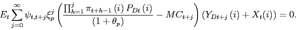$$\mathbb{E}_{t}\sum_{j=0}^{\infty}\psi_{t,t+j}\xi_{p}^{j}\left( \frac {\prod_{h=1}^{j}\pi_{t+h-1}\left( i\right) P_{Dt}\left( i\right) }{\left( 1+\theta_{p}\right) }-MC_{t+j}\right) (Y_{Dt+j}\left( i\right) +X_{t}(i))=0.$$ (6)

2.1.2  Production of the Domestic Output Index

Because households have identical Dixit-Stiglitz preferences, it is convenient to assume that a representative aggregator combines the differentiated intermediate products into a composite home-produced good $Y_{Dt}$:

$$Y_{Dt}=\left[ \int_{0}^{1}Y_{Dt}\left( i\right) ^{\frac{1}{1+\theta_{p}} }di\right] ^{1+\theta_{p}}.$$ (7)

The aggregator chooses the bundle of goods that minimizes the cost of producing $Y_{Dt}$, taking the price $P_{Dt}\left( i\right)$ of each intermediate good $Y_{Dt}(i)$ as given. The aggregator sells units of each sectoral output index at its unit cost $P_{Dt}$:

$$P_{Dt}=\left[ \int_{0}^{1}P_{Dt}\left( i\right) ^{\frac{-1\, \,}{\theta _{p}\,}}di\right] ^{-\theta_{p}}.$$ (8)

We also assume a representative aggregator in the North who combines the differentiated South products $X_{t}(i)$ into a single index for foreign imports:

$$M_{t}^{\ast}=\left[ \int_{0}^{1}X_{t}\left( i\right) ^{\frac{1} {1+\theta_{p}}}di\right] ^{1+\theta_{p}},$$ (9)

and sells $M_{t}^{\ast}$ at price $P_{Dt}.$

2.1.3  Production of Consumption and Investment Goods

Final consumption goods are produced by a representative consumption goods distributor. This firm combines purchases of domestically-produced goods with imported goods to produce a final consumption good ($C_{At})$ according to a constant-returns-to-scale CES production function:

$$C_{At}=\left( \omega_{C}^{\frac{\rho_{C}}{1+\rho_{C}}}C_{Dt}^{\frac{1} {1+\rho_{C}}}+(1-\omega_{C})^{\frac{\rho_{C}}{1+\rho_{C}}}(\varphi_{Ct} M_{Ct})^{\frac{1}{1+\rho_{C}}}\right) ^{1+\rho_{C}},$$ (10)

where $C_{Dt}$ denotes the consumption good distributor's demand for the index of domestically-produced goods, $M_{Ct}$ denotes the distributor's demand for the index of foreign-produced goods, and $\varphi_{Ct}$ reflects costs of adjusting consumption imports. The final consumption good is used by both households and by the government. The form of the production function mirrors the preferences of households and the government sector over consumption of domestically-produced goods and imports. Accordingly, the quasi-share parameter $\omega_{C}$ may be interpreted as determining the preferences of both the private and public sector for domestic relative to foreign consumption goods, or equivalently, the degree of home bias in consumption expenditure. Finally, the adjustment cost term $\varphi_{Ct}$ is assumed to take the quadratic form:

$$\varphi_{Ct}=\left[ 1-\frac{\varphi_{M_{C}}}{2}\left( \frac{\frac{M_{Ct} }{C_{Dt}}}{\frac{M_{Ct-1}}{C_{Dt-1}}}-1\right) ^{2}\right] .$$ (11)

This specification implies that it is costly to change the proportion of domestic and foreign goods in the aggregate consumption bundle, even though the level of imports may jump costlessly in response to changes in overall consumption demand.

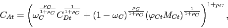
Given the presence of adjustment costs, the representative consumption goods distributor chooses (a contingency plan for) $C_{Dt}$ and $M_{Ct}$ to minimize its discounted expected costs of producing the aggregate consumption good:

$$\begin{align} & \min_{C_{Dt+k},M_{Ct+k}}\mathbb{E}_{t}\sum_{k=0}^{\infty}\psi_{t,t+k} \bigg \{ \left( P_{Dt+k}C_{Dt+k}+P_{Mt+k}M_{Ct+k}\right) \ & \left. +P_{Ct+k}\left[ C_{A,t+k}-\left( \omega_{C}^{\frac{\rho_{C} }{1+\rho_{C}}}C_{Dt+k}^{\frac{1}{1+\rho_{C}}}+(1-\omega_{C})^{\frac{\rho_{C} }{1+\rho_{C}}}(\varphi_{Ct+k}M_{Ct+k})^{\frac{1}{1+\rho_{C}}}\right) ^{1+\rho_{C}}\right] \right\} .\nonumber \end{align}$$ (12)

The distributor sells the final consumption good to households and the government at a price $P_{Ct}$, which may be interpreted as the consumption price index (or equivalently, as the shadow cost of producing an additional unit of the consumption good).

We model the production of final investment goods in an analogous manner, although we allow the weight $\omega_{I}$ in the investment index to differ from that of the weight $\omega_{C}$ in the consumption goods index.⁹

2.2  Households and Wage Setting

We assume a continuum of monopolistically competitive households (indexed on the unit interval), each of which supplies a differentiated labor service to the intermediate goods-producing sector (the only producers demanding labor services in our framework) following Erceg, Henderson and Levin (2000). A representative labor aggregator (or "employment agency") combines households' labor hours in the same proportions as firms would choose. Thus, the aggregator's demand for each household's labor is equal to the sum of firms' demands. The aggregate labor index $L_{t}$ has the Dixit-Stiglitz form:

$$L_{t}=\left[ \int_{0}^{1}\left( \zeta N_{t}\left( h\right) \right) ^{\frac{1}{1+\theta_{w}}}dh\right] ^{1+\theta_{w}},$$ (13)

where $\theta_{w}>0$ and $N_{t}(h)$ is hours worked by a typical member of household $h$. The parameter $\zeta$ is the size of a household of type $h$, and effectively determines the size of the population in the South. The aggregator minimizes the cost of producing a given amount of the aggregate labor index, taking each household's wage rate $W_{t}\left( h\right)$ as given, and then sells units of the labor index to the production sector at their unit cost $W_{t}$:

$$W_{t}=\left[ \int_{0}^{1}W_{t}{}\left( h\right) ^{\frac{-1}{\theta_{w}} }dh\right] ^{-\theta_{w}}.$$ (14)

The aggregator's demand for the labor services of a typical member of household $h$ is given by

$$N_{t}\left( h\right) =\left[ \frac{W_{t}\left( h\right) }{W_{t}}\right] ^{-\frac{1+\theta_{w}}{\theta_{w}}}L_{t}/\zeta.$$ (15)

We assume that there are two types of households: households that make intertemporal consumption, labor supply, and capital accumulation decisions in a forward-looking manner by maximizing utility subject to an intertemporal budget constraint (FL households, for "forward-looking"); and the remainder that simply consume their after-tax disposable income (HM households, for "hand-to-mouth" households). The latter type receive no capital rental income or profits, and choose to set their wage to be the average wage of optimizing households. We denote the share of FL households by 1-$\varsigma$ and the share of HM households by $\varsigma$.

We consider first the problem faced by FL households. The utility functional for an optimizing representative member of household $h$ is

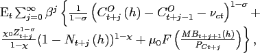$$\begin{align} & \mathbb{E}_{t}\sum_{j=0}^{\infty}\beta^{j}\left\{ \frac{1}{1-\sigma}\left( C_{t+j}^{O}\left( h\right) -\varkappa{C_{t+j-1}^{O}}-\nu_{ct}\right) ^{1-\sigma}+\right. \ & \left. \frac{\chi_{0}Z_{t+j}^{1-\sigma}}{1-\chi}(1-N_{t+j}\left( h\right) )^{1-\chi}+\mu_{0}F\left( \frac{MB_{t+j+1}(h)}{P_{Ct+j}}\right) \right\} ,\nonumber \end{align}$$ (16)

where the discount factor $\beta$ satisfies$\ 0<\beta<1.$ As in Smets and Wouters (2003, 2007), we allow for the possibility of external habit formation in preferences, so that each household member cares about its consumption relative to lagged aggregate consumption per capita of forward-looking agents $C_{t-1}^{O}$. The period utility function depends on an each member's current leisure $1-N_{t}\left( h\right)$, his end-of-period real money balances, $\frac{MB_{t+1}\left( h\right) }{P_{Ct}}$, and a preference shock, $\nu _{ct}$. The subutility function $F(.)$ over real balances is assumed to have a satiation point to account for the possibility of a zero nominal interest rate; see Eggertsson and Woodford (2003) for further discussion.¹⁰ The (log-linearized) consumption demand shock $\nu_{ct}$ is assumed to follow an AR(1) process:

$$\nu_{ct}=\rho_{\nu}\nu_{ct-1}+\varepsilon_{\nu_{c},t.}$$ (17)

Forward-looking household $h$ faces a flow budget constraint in period $t$ which states that its combined expenditure on goods and on the net accumulation of financial assets must equal its disposable income:

$$\begin{array}[c]{c} P_{Ct}\left( 1+\tau_{Ct}\right) C_{t}^{O}\left( h\right) +P_{It} I_{t}\left( h\right) +MB_{t+1}\left( h\right) -MB_{t}(h)+\int_{s} \xi_{t,t+1}B_{Dt+1}(h)\ -B_{Dt}(h)+P_{Bt}B_{Gt+1}-B_{Gt}+\frac{P_{Bt}^{\ast}B_{Ft+1}(h)}{\phi_{bt} }-B_{Ft}(h)\ =(1-\tau_{Nt})W_{t}\left( h\right) N_{t}\left( h\right) +\Gamma_{t}\left( h\right) +TR_{t}(h)+(1-\tau_{Kt})R_{Kt}K_{t}(h)+\ P_{It}\tau_{Kt}\delta K_{t}(h)-P_{Dt}\phi_{It}(h). \end{array}$$ (18)

Consumption purchases are subject to a sales tax of $\tau_{Ct}.$ Investment in physical capital augments the per capita capital stock $K_{t+1}(h)$ according to a linear transition law of the form:

$$K_{t+1}\left( h\right) =(1-\delta)K_{t}(h)+I_{t}(h),$$ (19)

where $\delta$ is the depreciation rate of capital.

Financial asset accumulation of a typical member of FL household $h$ consists of increases in nominal money holdings ( $MB_{t+1}\left( h\right) -MB_{t}\left( h\right) )$ and the net acquisition of bonds. While the domestic financial market is complete through the existence of state-contingent bonds $B_{Dt+1}$, cross-border asset trade is restricted to a single non-state contingent bond issued by the government of the North economy.¹¹

The terms $B_{Gt+1}$ and $B_{Ft+1}$ represents each household member's net purchases of the government bonds issued by the South and North governments, respectively. Each type of bond pays one currency unit (e.g., euro) in the subsequent period, and is sold at price (discount) of $P_{Bt}$ and $P_{Bt}^{\ast}$, respectively. To ensure the stationarity of foreign asset positions, we follow Turnovsky (1985) by assuming that domestic households must pay a transaction cost when trading in the foreign bond. The intermediation cost depends on the ratio of economy-wide holdings of net foreign assets to nominal GDP, $P_{t}Y_{t}$, and are given by:

$$\phi_{bt}=\exp\left( -\phi_{b}\left( \frac{B_{Ft+1}}{P_{t}Y_{t}}\right) \right) .$$ (20)

If the South is an overall net lender position internationally, then a household will earn a lower return on any holdings of foreign (i.e., North) bonds. By contrast, if the South has a net debtor position, a household will pay a higher return on its foreign liabilities. Given that the domestic government bond and foreign bond have the same payoff, the price faced by domestic residents net of the transaction cost is identical, so that $P_{Bt}=\frac{P_{Bt}^{\ast}}{\phi_{bt}}.$ The effective nominal interest rate on domestic bonds (and similarly for foreign bonds) hence equals $i_{t}=1/P_{Bt}-1$.

Each member of FL household $h$ earns after-tax labor income, $(1-\tau _{Nt})W_{t}\left( h\right) N_{t}\left( h\right)$, where $\tau_{Nt}$ is a stochastic tax on labor income. The household leases capital at the after-tax rental rate $(1-\tau_{Kt})R_{Kt}$, where $\tau_{Kt}$ is a stochastic tax on capital income. The household receives a depreciation write-off of $P_{It} \tau_{Kt}\delta$ per unit of capital. Each member also receives an aliquot share $\Gamma_{t}\left( h\right)$ of the profits of all firms and a lump-sum government transfer, $TR_{t}\left( h\right)$ (which is negative in the case of a tax). Following Christiano, Eichenbaum and Evans (2005), we assume that it is costly to change the level of gross investment from the previous period, so that the acceleration in the capital stock is penalized:

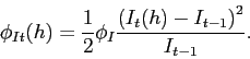$$\phi_{It}(h)=\frac{1}{2}\phi_{I}\frac{\left( I_{t}(h)-I_{t-1}\right) ^{2} }{I_{t-1}}.$$ (21)

In every period $t$, each member of FL household $h$ maximizes the utility functional (16) with respect to its consumption, investment, (end-of-period) capital stock, money balances, holdings of contingent claims, and holdings of domestic and foreign bonds, subject to its labor demand function (15), budget constraint (18), and transition equation for capital (19). In doing so, a household takes as given prices, taxes and transfers, and aggregate quantities such as lagged aggregate consumption and the aggregate net foreign asset position.

Forward-looking (FL) households set nominal wages in staggered contracts that are analogous to the price contracts described above. In particular, with probability $1-\xi_{w}$, each member of a household is allowed to reoptimize its wage contract. If a household is not allowed to optimize its wage rate, we assume each household member resets its wage according to:

$$W_{t}(h)=\omega_{t-1}^{\iota_{w}}\omega^{1-\iota_{w}}W_{t-1}(h),$$ (22)

where $\omega_{t-1}$ is the gross nominal wage inflation in period $t-1$, i.e. $W_{t}/W_{t-1}$, and $\omega=\pi$ is the steady state rate of change in the nominal wage (equal to gross price inflation since steady state gross productivity growth is assumed to be unity). Dynamic indexation of this form introduces some element of structural persistence into the wage-setting process. Each member of household $h$ chooses the value of $W_{t}(h)$ to maximize its utility functional (16) subject to these constraints.

Finally, we consider the determination of consumption and labor supply of the hand-to-mouth (HM) households. A typical member of a HM household simply equates his nominal consumption spending, $P_{Ct}\left( 1+\tau_{Ct}\right) C_{t}^{HM}\left( h\right)$, to his current after-tax disposable income, which consists of labor income plus lump-sum transfers from the government:

$$P_{Ct}\left( 1+\tau_{Ct}\right) C_{t}^{HM}\left( h\right) =(1-\tau _{Nt})W_{t}\left( h\right) N_{t}\left( h\right) +TR_{t}(h).$$ (23)

The HM households are assumed to set their wage equal to the average wage of the forward-looking households. Since HM households face the same labor demand schedule as the forward-looking households, this assumption implies that each HM household works the same number of hours as the average for forward-looking households.

2.3  Monetary Policy

We assume that the central bank follows a Taylor rule for setting the policy rate of the currency union, subject to the zero bound constraint on nominal interest rates. Thus:

$$i_{t}=\max\left\{ -i,\left( 1-\gamma_{i}\right) \left( \tilde{\pi} _{t}+\gamma_{\pi}(\tilde{\pi}_{t}-\pi)+\gamma_{x}\tilde{x}_{t}\right) +\gamma_{i}i_{t-1}\right\}$$ (24)

In this equation, $i_{t}$ is the quarterly nominal interest rate expressed in deviation from its steady state value of $i$. Hence, imposing the zero lower bound implies that $i_{t}$ cannot fall below $-i.$ $\tilde{\pi}_{t}$ is price inflation rate of the currency union, $\pi$ the inflation target, and $\tilde{x}_{t}$ is the output gap of the currency union. The aggregate inflation and output gap measures are defined as a GDP-weighted average of the inflation rates and output gaps of the South and North. Finally, the output gap in each member is defined as the deviation of actual output from its potential level, where potential is the level of output that would prevail if wages and prices were completely flexible.

2.4  Fiscal Policy

Intertemporal Budget Constraint The government does not need to balance its budget each period, and issues nominal debt $B_{Gt+1}$ at the end of period $t$ to finance its deficits according to:

$$\begin{array}[c]{c} P_{Bt}B_{Gt+1}-B_{Gt}=P_{Ct}G_{t}+TR_{t}-\tau_{Nt}W_{t}L_{t}-\tau_{Ct} P_{Ct}C_{t}-(\tau_{Kt}R_{Kt}-\delta P_{It})K_{t}\ -(MB_{t+1}-MB_{t}), \end{array}$$ (25)

where $C_{t}$ is total private consumption. Equation (25) aggregates the capital stock, money and bond holdings, and transfers and taxes over all households so that, for example, $TR_{t}=\int_{0}^{1}TR_{t}(h)dh$. The taxes on capital $\tau_{Kt}$ and consumption $\tau_{Ct}$ are assumed to be fixed, and the ratio of real transfers to (trend) GDP, $tr_{t}=\frac{TR_{t} }{P_{t}Y}$, is also fixed.¹² Government purchases have no direct effect on the utility of households, nor do they affect the production function of the private sector.

Alternative Approaches to Fiscal Consolidation We assume that policymakers adjust spending or taxes to keep both the debt/GDP ratio and the deficit close to a target path. If government spending is the fiscal instrument, we assume that spending adjusts endogenously according to the rule:

$$g_{t}=\nu_{g_{0}}g_{t-1}+\left( 1-\nu_{g_{0}}\right) \left[ \nu_{g_{1} }\left( b_{Gt}-b_{Gt}^{\ast}\right) +\nu_{g_{2}}\left( \Delta b_{Gt+1}-\Delta b_{Gt+1}^{\ast}\right) \right] .$$ (26)

In this equation, $g_{t}$ is the percent deviation of government spending from its steady state level, $b_{Gt}$ is the ratio of actual nominal debt to steady state (or "trend") nominal GDP, and $b_{Gt}^{\ast}$ the target debt/GDP ratio.¹³ The labor income tax rate is assumed to be constant if the government follows this rule (at its steady state value of $\tau_{N}).$ Alternatively, if the labor tax is the fiscal instrument, the labor tax rate evolves according to:

$$\tau_{Nt}-\tau_{N}=\nu_{\tau_{0}}\left( \tau_{Nt-1}-\tau_{N}\right) +\left( 1-\nu_{\tau_{0}}\right) \left[ \nu_{\tau_{1}}(b_{Gt}-b_{Gt}^{\ast} )+\nu_{\tau_{2}}(\Delta b_{Gt+1}-\Delta b_{Gt+1}^{\ast})\right] .$$ (27)

When the government adopts the labor income tax based consolidation strategy, real government spending $g_{t}$ is assumed to be unchanged from steady state (i.e., $g_{t}$ = 0); of course, this implies that the government spending share of actual output must vary. Under either fiscal rule, real government transfers $tr_{t}$ are also held constant at steady state (implying that the ratio of transfers to actual GDP varies countercyclically).

Our main simulations assume that the government in the South desires to reduce its debt target $b_{Gt}^{\ast}.$ It is realistic to assume that policymakers would reduce the debt target gradually to help avoid potentially large adverse consequences on output. To capture this gradualism, we assume that the (end of period $t)$ debt target $b_{Gt+1}^{\ast}$ follows an AR(2) process:

$$b_{Gt+1}^{\ast}-b_{Gt}^{\ast}=\rho_{d_{1}}(b_{Gt}^{\ast}-b_{Gt-1}^{\ast} )-\rho_{d_{2}}b_{Gt}^{\ast}+\varepsilon_{d^{\ast},t},$$ (28)

where $0\leq\rho_{d_{1}}<1$ and $\rho_{d_{2}}>0$.

The North is assumed to simply follow an endogenous tax rule as in (27), but does not change its debt target.

2.5  Resource Constraint and Net Foreign Assets

The domestic economy's aggregate resource constraint can be written as:

$$Y_{Dt}=C_{Dt}+I_{Dt}+\phi_{It},$$ (29)

where $\phi_{It}$ is the adjustment cost on investment aggregated across all households. The final consumption good is allocated between households and the government:

$$C_{At}=C_{t}+G_{t},$$ (30)

where $C_{t}$ is total private consumption of FL (optimizing) and HM households:

$$C_{t}=C_{t}^{O}+C_{t}^{HM}.$$ (31)

Total exports may be allocated to either the consumption or the investment sector abroad:

$$M_{t}^{\ast}=M_{Ct}^{\ast}+M_{It}^{\ast}.$$ (32)

Finally, at the level of the individual firm:

$$Y_{t}(i)=Y_{Dt}(i)+X_{t}(i)\, \, \, \, \, \, \, \, \forall i.$$ (33)

The evolution of net foreign assets can be expressed as:

$$\frac{P_{B,t}^{\ast}B_{F,t+1}}{\phi_{bt}}=B_{F,t}+P_{Mt}^{\ast}M_{t}^{\ast }-P_{Mt}M_{t}.$$ (34)

This expression can be derived from the budget constraint of the FL households after imposing the government budget constraint, the consumption rule of the HM households, the definition of firm profits, and the condition that domesticstate-contingent non-government bonds ($B_{Dt+1}$) are in zero net supply.

Finally, we assume that the structure of the foreign country (the North) is isomorphic to that of the home country (the South).

2.6  Production of Capital Services

We incorporate a financial accelerator mechanism into both country blocks of our benchmark model following the basic approach of Bernanke, Gertler and Gilchrist (1999). Thus, the intermediate goods producers rent capital services from entrepreneurs (at the price $R_{Kt})$ rather than directly from households. Entrepreneurs purchase physical capital from competitive capital goods producers (and resell it back at the end of each period), with the latter employing the same technology to transform investment goods into finished capital goods as described by equations 19) and 21). To finance the acquisition of physical capital, each entrepreneur combines his net worth with a loan from a bank, for which the entrepreneur must pay an external finance premium (over the risk-free interest rate set by the central bank) due to an agency problem. Banks obtain funds to lend to the entrepreneurs by issuing deposits to households at the interest rate set by the central bank, with households bearing no credit risk (reflecting assumptions about free competition in banking and the ability of banks to diversify their portfolios). In equilibrium, shocks that affect entrepreneurial net worth - i.e., the leverage of the corporate sector - induce fluctuations in the corporate finance premium.¹⁴

3.  Solution Method and Calibration

To analyze the behavior of the model, we log-linearize the model's equations around the non-stochastic steady state. Nominal variables are rendered stationary by suitable transformations. To solve the unconstrained version of the model, we compute the reduced-form solution of the model for a given set of parameters using the numerical algorithm of Anderson and Moore (1985), which provides an efficient implementation of the solution method proposed by Blanchard and Kahn (1980). When we solve the model subject to the non-linear monetary policy rule (24), we use the techniques described in Hebden, Lindé and Svensson (2009). An important feature of the Hebden, Lindé and Svensson algorithm is that the duration of the liquidity trap is endogenously determined.¹⁵

The model is calibrated at a quarterly frequency. Structural parameters are set at identical values for each of the two country blocks, except for the parameter $\zeta$ determining population size (as discussed below), the fiscal rule parameters, and the parameters determining trade shares. We assume that the discount factor $\beta=0.995$, consistent with a steady-state annualized real interest rate $\overline{r}$ of 2 percent. By assuming that gross inflation $\pi=1.005$ (i.e., a net inflation of 2 percent in annualized terms), the implied steady state nominal interest rate $i$ equals 0.01 at a quarterly rate, and 4 percent at an annualized rate.

The utility functional parameter $\sigma$ is set equal to 1 to ensure that the model exhibit balanced growth, while the parameter determining the degree of habit persistence in consumption $\varkappa=0.8$. We set $\chi=4$, implying a Frisch elasticity of labor supply of 1/2, which is roughly consistent with the evidence reported by Domeij and Flodén (2006). The utility parameter $\chi_{0}$ is set so that employment comprises one-third of the household's time endowment, while the parameter $\mu_{0}$ on the subutility function for real balances is set at an arbitrarily low value (so that variation in real balances do not affect equilibrium allocations). We set the share of HM agents $\varsigma=0.47,$ implying that these agents account for about 20 percent of aggregate private consumption spending (the latter is much smaller than the population share of HM agents because the latter own no capital).

The depreciation rate of capital $\delta$ is set at 0.03 (consistent with an annual depreciation rate of 12 percent). The parameter $\rho$ in the CES production function of the intermediate goods producers is set to -2, implying an elasticity of substitution between capital and labor $(1+\rho)/\rho$, of 1/2. The quasi-capital share parameter $\omega_{K}$ - together with the price markup parameter of $\theta_{P}=0.20$ - is chosen to imply a steady state investment to output ratio of 15 percent. We set the cost of adjusting investment parameter $\phi_{I}=3$, slightly below the value estimated by Christiano, Eichenbaum and Evans (2005). The calibration of the parameters determining the financial accelerator follows Bernanke, Gertler and Gilchrist (1999). In particular, the monitoring cost, $\mu$, expressed as a proportion of entrepreneurs' total gross revenue, is set to 0.12. The default rate of entrepreneurs is 3 percent per year, and the variance of the idiosyncratic productivity shocks to entrepreneurs is 0.28.

Our calibration of the parameters of the monetary policy rule and the Calvo price and wage contract duration parameters - while within the range of empirical estimates - tilt in the direction of reducing the sensitivity of inflation to shocks. These choices seem reasonable given the resilience of inflation in most euro area countries in the aftermath of the global financial crisis. In particular, we set the parameters of the monetary rule such that $\gamma_{\pi}=1.5$, $\gamma_{x}=0.125$, and $\gamma_{i}=0.7,$ implying a considerably larger response to inflation than a standard Taylor rule (which would set $\gamma_{\pi}=0.5).$ The price contract duration parameter $\xi_{p}=0.9,$ and the price indexation parameter $\iota_{p}=0.65$. Our choice of $\xi_{p}$ implies a Phillips curve slope of about 0.007 which is a bit lower than the median estimates in the literature that cluster in the range of 0.009 - 0.014, but well within the standard confidence intervals provided by empirical studies (see e.g. Adolfson et al (2005), Altig et al. (2010), Galí and Gertler (1999), Galí, Gertler, and López-Salido (2001), Lindé (2005), and Smets and Wouters (2003, 2007)). Our choices of a wage markup of $\theta_{W}$ = $1/3,$ a wage contract duration parameter of $\xi_{w}=0.85,$ and a wage indexation parameter of $\iota_{w}=0.65,$ together imply that wage inflation is about as responsive to the wage markup as price inflation is to the price markup.¹⁶

The parameters pertaining to fiscal policy are intended to roughly capture the revenue and spending sides of euro area government budgets. The share of government spending on goods and services is set equal to 23 percent of steady state output. The government debt to GDP ratio, $b_{G}$, is set to 0.75, roughly equal to the average level of debt in euro area countries at end-2008. The ratio of transfers to GDP is set to 20 percent. The steady state sales (i.e., VAT) tax rate $\tau_{C}$ is set to 0.2, while the capital tax $\tau_{K}$ is set to 0.30. Given the annualized steady state real interest rate (2 percent), the government's intertemporal budget constraint then implies that the labor income tax rate $\tau_{N}$ equals 0.42 in steady state. The coefficients of the spending and tax adjustment rules $\left\{ \nu_{g_{1}},\nu_{\tau_{1}}\right\}$ and $\left\{ \nu_{g_{2}} ,\nu_{\tau_{2}}\right\}$ in equations (26) and (27) for the South are set such that the fiscal instrument - either $g_{t}$ or $\tau_{Nt}$ - in the long-run is decreased (increased) by 0.5 and 0.25 percent of trend GDP, respectively, in response to one-percentage point target deviations from debt ( $b_{Gt} -b_{Gt}^{\ast}$) and deficit $(\Delta b_{Gt+1}-\Delta b_{Gt+1}^{\ast});$ we also allow for a small degree of inertia, so that $\nu_{g_{0}}=\nu_{\tau_{0} }=0.5$. These coefficients imply that the debt/GDP ratio essentially converges to target after three years following a target shock (i.e., to $b_{Gt}^{\ast})$ in the flexible price and wage variant of the model. For the North, we assume an unaggressive tax rule, which is achieved by setting $\nu_{\tau_{0}}=0.985$ and $\nu_{\tau_{1}}=\nu_{\tau_{2}}=.1$.

The size of the South is calibrated to be 1/3 of euro area GDP, so that $\zeta=0.5.$ This corresponds to the collective share of Greece, Ireland, Portugal, Italy, and Spain in euro area GDP, or alternatively, to the combined GDP of France and Spain (clearly, our model framework can be applied to many other country pairings, with similar implications). Identifying the former group of countries as the South to calibrate trade shares, the average share of imports of the South from the remaining countries of the euro area was about 14 percent of GDP in 2008 (based on Eurostat). This pins down the trade share parameters $\omega_{C}$ and $\omega_{I}$ for the South under the additional assumption that the import intensity of consumption is equal to 3/4 that of investment. Given that trade is balanced in steady state, this calibration implies an export and import share of the North countries of 7 percent of GDP.

We assume that $\rho_{C}=\rho_{I}=2$, consistent with a long-run price elasticity of demand for imported consumption and investment goods of 1.5. The adjustment cost parameters are set so that $\varphi_{M_{C}} =\varphi_{M_{I}}=1$, which slightly damps the near-term relative price sensitivity. The financial intermediation parameter $\phi_{b}$ is set to a very small value (0.00001), which is sufficient to ensure the model has a unique steady state.

Finally, the persistence coefficient $\rho_{\nu_{c}}$ for the consumption demand shock $\nu_{ct}$ (see eq.17) is set to 0.9, while the persistence coefficient $\rho_{z}$ for the technology shock (see eq. 4) assumes the value 0.975.

4.  Benchmark Results

In this section, we report the results under our benchmark calibration.

4.1  Fiscal Consolidation: Independent Monetary Policy and Currency Union

Our baseline simulations involve comparing the effects of a 25 percent reduction in the desired long-run debt target $b_{Gt}^{\ast}$ in the South that is achieved either through a spending cut or tax hike. The parameters of the debt target evolution equation (28) are set so that $\rho_{d_{1}}=0.935$ and $\rho_{d_{2}}=0.0001$, implying that about half of the convergence to the new long-run debt target is achieved after three years, and that the debt target is (virtually) fully implemented after 10 years. The debt target path is shown by the dashed line in panel 8 of Figure 1.¹⁷

To assess the impact of various constraints on monetary and exchange rate adjustment, it is useful to first consider the case of an independent monetary policy (IMP) - unconstrained by the zero lower bound and currency union membership - as a reference point. In that vein, the solid lines in Figure 6 show impulse responses to the change in the debt target under an IMP, both under a spending-based consolidation, as determined by the spending rule given by equation (26), and for a tax-based consolidation as determined by equation (27). Under the IMP, the South has a floating exchange rate with the North. Moreover, both the South and North are assumed to adjust policy rates according to the Taylor rule in equation (24), except that aggregate inflation and output gap measures are replaced with country-specific variables.

Consistent with the empirical findings of Alesina and Perotti (1995, 1997), Figure 1 shows that a spending-based consolidation (thick solid lines) has considerably smaller adverse effects on output than a tax-based consolidation (thin solid lines) in this case. Given that monetary policy keeps output reasonably close to potential under either form of consolidation, the disparity in the output responses largely reflects differences in the response of potential output (panel 6). In particular, the persistent rise in the labor tax rate (panel 10) has a large and protracted adverse effect on potential output, as higher taxes reduce both labor supply and capital spending. By contrast, the effects of the government spending shock on potential are much smaller in magnitude, and more transient (potential falls in the latter case due to adverse effects on labor supply that are most pronounced when government spending troughs 2-3 years after the debt target shock).¹⁸

Defining the "fiscal sacrifice ratio" as the cost of reducing public debt by one percentage point of GDP, it is clear that the fiscal sacrifice ratio associated with spending cuts is much lower than under tax-based consolidation even at relatively short horizons. For example, with a tax hike, output falls 2 percent after two years, while the debt/GDP ratio is reduced about 4 percentage points, consistent with a "fiscal sacrifice ratio" of 1/2 at a two year horizon. By contrast, output falls only about half as much under the spending-based consolidation, while progress in reducing debt is slightly faster, implying a sacrifice ratio of less than 1/4. At somewhat longer horizons, the comparative advantage of spending cuts - in terms of producing a relatively lower fiscal sacrifice ratio - is even more pronounced.

The spending-based consolidation requires monetary policy in the South to cut interest rates (panel 1) sharply in order to keep output near potential, and inflation near target. These interest rate cuts induce "crowding in" effects on household consumption and business investment (as the cost-of capital falls). In addition, the exchange rate depreciates - both in response to lower interest rates and because lower government spending increases the supply of domestic goods available for alternative uses - which in turn boosts real net exports.

In the case of the tax-based consolidation, the South would also cut interest rates in the near-term to help keep output near potential (under an IMP). Several factors put initial downward pressure on interest rates, including that the hand-to-mouth households experience a direct fall in their after-tax income, that Ricardian households expect their consumption to grow slowly in the near-term (as higher taxes depress potential output growth), and that falling employment reduces investment demand. However, the magnitude and persistence of the decline in interest rates required to keep output near potential is much smaller than in the case of spending cuts (implying that long-term interest rates don't fall nearly as much). In fact, interest rates (panel 1) begin to rise after a few years as the expectation that tax rates (panel 10) will begin falling towards their pre-shock level induces households to expect their consumption will rebound. Despite putting modest downward pressure on interest rates, the tax-based consolidation causes the real exchange rate to appreciate, reflecting the fall in the relative supply of the South's goods.

We next compare the different approaches to fiscal consolidation under our benchmark model which assumes that the South is part of a currency union (CU) with the North. As seen from the dashed lines in Figure 6, these results are quite different than under an IMP, as an expenditure-based consolidation depresses output (panel 5) by more than a tax-based consolidation for several years. Two factors account for the large output decline under the expenditure-based consolidation. First, while spending cuts require large and persistent interest rate declines to crowd-in private demand and keep output near potential, the CU central bank provides too little accommodation given its focus on union-wide aggregates. Second, the nominal exchange rate remains fixed, rather than depreciating as in the case of an IMP, which reduces the near-term stimulus to real net exportsas it takes time for the real exchange rate to appreciate given that both prices and wages are sticky.

By contrast, the response of output to the tax-based consolidation is broadly similar across the two regimes. Perhaps surprisingly, output even falls a bit less under a CU than under an IMP. Because the nominal exchange rate is fixed under a CU, the real exchange rate appreciates gradually (panel 3) - rather than jumping as under an IMP - which serves to dampen the contractionary impact on real net exports. Moreover, the behavior of real interest rates turns out to be quite similar across the two regimes. Although nominal interest rates fall by less under a CU than under an IMP at a horizon extending out several years, inflation rises under a CU, instead of falling as under an IMP. The higher inflation reflects that the price of the South's goods relative to the North's must rise, and that CU monetary policy comes close to stabilizing the average inflation rate in the CU (so that the relative price increase must translate into higher inflation in South for some time). Finally, interest rates rise by less in the longer-term under a CU than under an IMP.

Under a CU, the larger output contraction in response to an expenditure-based consolidation translates into less initial progress in reducing the debt/GDP ratio, and a correspondingly higher fiscal sacrifice ratio; in fact, the debt/GDP ratio rises for about two years. Even so, because real interest rates and real exchange rates gradually adjust towards their flexible price levels at longer horizons, the sacrifice ratio associated with a spending-based consolidation eventually falls below that of a tax-based consolidation, with the cross-over occurring after three years under our benchmark calibration. Thus, the CU constraint in effect introduces an intertemporal trade-off between tax-based and expenditure-based consolidation. The output contraction is smaller under tax-based consolidation in the near-term, but is a considerably deeper at longer horizons.

4.2  Fiscal Consolidation in Currency Union (Unconstrained and ZLB)

4.2.1  Initial Conditions for Liquidity Trap

We next examine the effects of the alternative approaches to fiscal consolidation when the CU itself is constrained by a liquidity trap. We generate a liquidity trap by specifying initial conditions that are consistent with a deep recession. In particular, we assume that negative taste and technology shocks in both South and North generate a sharp fall in output and inflation as shown by the solid lines in Figure 6, and cause the policy rate to decline to its lower bound of zero for eight quarters. The shocks are scaled to induce a maximum output contraction of 10 percent relative to baseline, which is similar to the decline in euro area GDP between end-2007 and end-2011 relative to its pre-2007 trend. The negative technology shock also implies that the fall in output relative to it pre-crisis trend is highly persistent, a feature which is consistent with historical evidence for banking and financial crises (e.g. Reinhart and Rogoff, 2008). The large and persistent fall in output implies that government tax revenues fall and spending increase (as share of GDP), triggering a persistent primary deficit and higher debt service costs. This puts substantial upward pressure on government debt, which would rise above 100 percent of GDP after 10 years absent any fiscal actions (though the labor tax rate eventually adjusts to stabilize the debt/GDP at its pre-crisis level).¹⁹

4.2.2  Effects of Fiscal Consolidation

Figure 6 compares the responses when monetary policy in the currency union ("Normal") is unconstrained - as in Figure 6 - with a situation where the currency union is constrained by a liquidity trap that would last eight quarters in the absence of fiscal actions (i.e., the baseline in Figure 6). Specifically, the impulse response functions shown in Figure 6 are computed as the difference between the scenario which includes both the baseline shocks and fiscal austerity measures, and the scenario with only the baseline shocks in Figure 6. The austerity measures are assumed to be announced and implemented in the first period the ZLB actually binds, i.e. period 4 in Figure 6.²⁰

Clearly, the adverse impact of a spending-based consolidation on output (solid thick line in panel 5) is exacerbated considerably when the CU central bank is constrained by the ZLB. The magnitude of the output contraction is roughly three times larger when the CU is constrained by the ZLB than when it is unconstrained. The much larger output contraction when the ZLB is binding reflects several factors. First, the endogenous decline in government spending (panel 9) is significantly larger, reflecting that the slow progress in reducing the debt/GDP ratio (panel 8) prompts much deeper spending cuts. Second - as we explore in more detail below - because the large spending cuts stretch the duration of the liquidity trap to 12 quarters, they have increasingly negative effects on output at the margin. Finally, the spillover effects to the North (panel 7) become substantially negative, which tends to hurt the South's exports (offsetting the stimulus from exchange rate depreciation, as seen in panel 3). The contraction in is in stark contrast to normal conditions in which the CU central bank would lower policy rates enough to boost the North's output (dashed thick line in panel 7), and by so doing would help stabilize the CU-wide output gap and inflation rate. Given that policy rates are constrained in the liquidity trap and inflation falls even in the North, higher real interest rates depress the North's domestic demand.²¹

The sharp output decline in response to the expenditure-based consolidation in the South actually causes its debt/GDP ratio to rise by around 7 percentage points after two years. No noticeable progress occurs in reducing debt until about four years into the consolidation.

As seen in Figure 3, the ZLB also amplifies the contractionary impact of a tax-based consolidation on output (panel 5) relative to the case in which the CU is unconstrained. With a binding ZLB, the real interest rate is higher, which reduces private absorption; and demand from the North is also somewhat weaker. The higher real interest rate in turn reflects the delayed adjustment of the nominal interest rate relative to the unconstrained case (panel 1). In addition, because the ZLB precludes the CU central bank from offsetting the downward initial pressure on CU aggregate demand arising from the South's tax consolidation, inflation falls even in the South (in contrast to the rise when the CU is unconstrained). Real interest rates also rise in the North, compressing domestic demand and hence the South's exports.²²

Although the contractionary impact of the ZLB becomes more pronounced as the liquidity trap deepens - as we show in the next section - the striking aspect of Figure 3 is how little the ZLB augments the output effects of the 25 percent of GDP tax-based consolidation relative to the amplification under the same-sized spending-based consolidation. For the tax consolidation, the output response is only amplified bya factor of 1.1 - 1.15, and is in fact very close to the output response under an IMP. While CU membership provides too little near-term monetary stimulus relative to an IMP - especially if the CU is in a liquidity trap - this is counterbalanced by a relatively smaller rise in interest rates at longer horizons. Moreover, the CU prevents the nominal exchange rate from immediately appreciating, which also provides some stimulus.

Because the effects of the tax-based consolidation are only slightly more negative in the liquidity trap case thanwhen the CU is unconstrained, the tax-based consolidation is much more effective than the spending-based consolidation in reducing the debt/GDP ratio out to a horizon of about 5 years. The tax-based consolidation also has comparatively modest negative spillover effects to the North. It is only at horizons beyond five years that the fiscal sacrifice ratio associated with reducing expenditure falls below that associated with tax cuts, reflecting that the eventual exit from the liquidity trap allows CU monetary policy much greater latitude to cushion the impact of spending cuts.

Although we do not examine sales taxes explicitly in this paper, it seems likely that the implications for consolidation would be fairly similar to labor taxes, and possibly even a bit more favorable. A higher sales tax is similar to a higher labor tax insofar as each reduces the after-tax return to working, which depresses potential output, and has an immediate depressing effect on the consumption of HM agents. However, as argued by Feldstein (2002), sales taxes also affect the intertemporal price of consumption, which gives policymakers a potentially important lever through which to affect aggregate demand. Based on related analysis by Correia, Nicolini, and Teles (2008) in a stylized closed economy New Keynesian model, it seems plausible that a consolidation involving both sales and labor tax rates could be even better suited to mitigating the monetary constraints we consider than the labor tax alone.

Figure 6 helps understand the channels through which the government expenditure cuts cause the debt/GDP ratio to rise for several years.²³ In particular, the solid lines in the upper panel show the response of the debt/GDP ratio if the CU is unconstrained, along with a decomposition of the cumulative sources of improvement at intervals ranging from 4-20 quarters; the lower panel presents analogous results for the case in which the CU is in a liquidity trap. Because the government spending cuts are highly persistent, its (cumulative) contribution -- shown by the yellow bars in each panel - becomes progressively more negative. As expected, the effects of spending cuts ceteris paribus is to reduce debt. However, falling labor and capital tax revenues offset a substantial part of the decline in the debt/GDP ratio attributable directly to the spending cuts, especially so when the CU is constrained by the ZLB. Moreover, the much larger fall in inflation in a liquidity trap drives a substantial rise in debt servicing costs as a share of GDP (red bars), which also contributes substantially to the initial runup in the debt/GDP ratio at a horizon of 4-12 quarters. Finally, the negative GDP response also has a direct impact on the debt to actual GDP ratio, as indicated by the differences between the debt to actual GDP (dot-solid) and debt to trend GDP (cross-dashed) lines. This effect is particularly important in a liquidity trap, when the adverse impact on GDP is substantially larger.

Our model assumes that the government issues only one period nominal bonds. If we allowed for longer maturity nominal debt, it seems likely that the government debt/GDP ratio would rise considerably more under the spending-based consolidation given the substantial deflationary impact of the shock; in our setting, lower short-term interest rates help restrain some of the upward pressure on the debt/GDP ratio.

4.3  Marginal Effects of Taxes vs. Spending

If the CU central bank was unconstrained by the ZLB, the effects of fiscal consolidation of either type would simply vary linearly with the size of the consolidation. However, fiscal consolidation can potentially have effects on output that become progressively more contractionary at the margin if the CU central bank is constrained by the ZLB. In such an environment, fiscal consolidation by a relatively large economy in a currency union (or consolidation undertaken by a group of economies) can depress aggregate, or CU-wide, output and inflation by enough to extend the duration of the liquidity trap faced by the CU, thereby causing fiscal consolidation to become more contractionary at the margin. Thus, while fiscal consolidation by a small economy has a small impact on CU aggregates and thus approximately has linear effects, it is important to consider how the effects of fiscal consolidation vary with scale in our case when the South is calibrated to constitute a large economy or group of economies.

To examine how the effects of fiscal consolidation vary with scale, Figure 6 plots the effects of different-sized spending based consolidations in which the debt target is lowered by 5, 15, and 25 percentage points (our benchmark), with the left column showing spending-based consolidation, and the right column tax-based consolidation. The fiscal consolidation is taken against the backdrop of the initial conditions shown in Figure 2 with an eight quarter liquidity trap (though the figure also reports the effects under a 5 percentage point cut when CU monetary policy is unconstrained as a reference point). The impact of the spending cuts on output (panel 3) are clearly nonlinear; notably, the 25 percentage point cut causes output to contract more than three times as much as the 15 percentage point cut. Moreover, the debt/GDP ratio falls in the near-term with the smaller fiscal consolidation - reflecting the relatively small output multiplier - but rises for the larger-sized consolidation. By contrast, the effects of progressively larger tax-based consolidations on output and government debt are close to linear over the range of consolidation sizes considered.

The much greater degree of nonlinearity for spending cuts rather than tax hikes reflects that the former require a much greater degree of monetary accommodation to keep output near potential; because policy rates cannot be cut immediately, the spending cuts prolong the liquidity trap, making additional spending cuts even more costly at the margin. Thus, as seen in Figure 6, the 25 percentage point spending cut extends the liquidity trap by four quarters relative to the case of a 5 percentage point contraction (panel 11).²⁴ It bears emphasizing, however, that even a tax-based consolidation puts downward pressure on the potential real interest rate in the near-term through the channels discussed above, including by temporarily depressing both household consumption demand and business investment. Because the drag on aggregate demand tends to be smaller for a given-sized tax-based consolidation (reflecting that e.g., households project that tax rates will eventually fall back towards baseline), much larger consolidations are required for these effects to become apparent relative to the case of spending-based consolidations.

In this vein, the upper panel of Figure 6 illustrates how the effects of each type of consolidation on output and the government debt/GDP ratio vary with the duration of the liquidity trap under our benchmark calibration. Following Erceg and Lindé (2010b), the multipliers shown are "marginal" multipliers in the sense that they show the impact of a "tiny" change in the fiscal instrument (spending or tax rates) that is small enough to keep the liquidity trap duration fixed at the level shown on the horizontal axis. The figure reports a three year discounted present value multiplier following Uhlig (2010), and hence is computed by setting $K=12$ in the formula:

$$m_{K}^{y}=\mathbf{\ }\frac{1}{fi_{y}}\frac{\frac{1}{K}\sum_{k=0}^{K-1} \beta^{k}\Delta y_{t+k}}{\frac{1}{K}\sum_{k=0}^{K-1}\beta^{k}\Delta fi_{t+k}},$$ (35)

i.e., as the discounted increment in output to the discounted change in the fiscal instrument $fi_{t+k}$ (both instruments expressed as share of trend output, $fi_{y}$), where $\Delta$ indicates an infinitesimal increase in the fiscal instrument. As seen in the figure, the multiplier schedules for both spending and tax consolidations follow a step function: the multiplier is constant until government spending cuts (or labor tax hikes) cumulate to a threshold value that is large enough to extend the liquidity trap by one quarter; beyond this value, the multiplier jumps discretely. The marginal debt multiplier is defined as the change in debt at a horizon of $K$ quarters ($K=12$) associated with an infinitesmal change in the undiscounted fiscal instrument:

$$m_{K}^{debt}=\mathbf{\ }\frac{1}{fi_{y}}\frac{\Delta b_{Gt+K}}{\frac{1}{K} \sum_{k=0}^{K-1}\Delta fi_{t+k}}.$$ (36)

The economic interpretation of the multiplier schedules is that progressively larger consolidation - by lengthening the duration of the liquidity trap, and thus reducing the latitude for future monetary accommodation - has a larger adverse impact on output at the margin. Thus, tax-based as well as spending-based consolidations have increasingly adverse effects if they are large enough in scale; as discussed in Erceg and Lindé (2010b), the convexity in the schedules reflects larger effects on expected inflation in a prolonged liquidity trap. Even so, the tax multiplier clearly rises much less abruptly with the duration of the liquidity trap than the spending multiplier; and the liquidity trap duration also varies much less with the size of consolidation (as apparent from the policy rate responses in Figure 5). These features together account for why the output impulse responses in Figure 5 appear highly nonlinear when the consolidation is spending based - in which case the liquidity trap is extended four quarters by the 25 percentage point debt target cut - but close to linear for tax based consolidations - in which case the liquidity trap duration only increases one quarter.

The contour of the multiplier schedule has important implications for how fiscal consolidation affects the government debt/GDP ratio. As seen in the upper right panel, spending cuts associated with a shorter-lived liquidity trap (either because the cuts are small, or because initial conditions facing the CU are relatively favorable) generate a substantial fall in government debt at the margin at the 3-year horizon (consistent with the unconstrained CU results in Figure 6).²⁵ By contrast, spending cuts associated with a deep liquidity trap actually cause debt to rise, reflecting that the highly adverse effects on output reduce tax revenue and raise debt servicing costs; for example, in an 11 quarter liquidity trap, a one percentage point average decline in spending relative to baseline causes government debt to increase by 3 percentage points relative to baseline at a 3-year horizon. The shift in the sign of the marginal government debt multiplier helps account for why the impulse response of government debt to the 25 percentage point fiscal contraction in Figure 5 is substantially positive (with government debt rising 7 percentage points). By contrast, given that tax-based consolidation has much smaller output effects, the government debt multiplier schedule rises much less abruptly as the liquidity trap duration increases, and implies that tax hikes reduce debt even in a long-lived liquidity trap of 11 quarters.

The contours of these schedules also depend importantly on the degree of price and wage rigidity in the economy. As noted earlier, our baseline calibration is already tilted toward the low end of empirical estimates of the sensitivity of price inflation to marginal cost, and of wage inflation to the wage markup. Even so, the resilience of inflation during the global recession and its aftermath suggests that the responsiveness of inflation may be even less than in our baseline. Accordingly, it is of interest to examine an alternative calibration with a higher degree of price and wage stickiness which sets $\xi_{p}=0.95$ and $\xi_{w}=0.9;$ the implied sensitivity of inflation to marginal cost is .002, far below the range of empirical estimates. The output multiplier is clearly smaller in the lower panel for any liquidity trap duration, reflecting that expected inflation falls much less when spending is cut. Thus, the consequences of a spending-based consolidation for the debt/GDP ratio are considerably more favorable than under our benchmark calibration (comparing the lower with the upper right panel). Even so, the marginal spending multiplier still lies uniformly above the tax multiplier, and rises more abruptly as the liquidity trap duration lengthens; thus, spending-based consolidations would still be more costly in the near-term even under very sluggish price adjustment, though the disparity between the approaches clearly narrows.²⁶

4.4  Mixed Strategies

Thus far, we have considered consolidation strategies that rely exclusively on either spending cuts or tax hikes. However, given that tax-based consolidations are relatively attractive in the near-term if monetary policy is constrained, while spending-based consolidations induce a smaller longer-term output contraction, a "mixed strategy" that combines sharp but temporary tax increases with more gradual spending cuts has obvious appeal. The work of Eggertsson (2010) and Christiano, Eichenbaum and Rebelo (2011), who argue that temporary tax hikes can in fact cause output to expand, also suggests the promise of such a strategy. On the spending side, the work of Cogan et al. (2010), Erceg and Lindé (2010b) and Corsetti, Kuester, Meier and Müller (2010b) highlights the merits of phasing-in expenditure cuts to mitigate adverse effects on output, especially if possibilities for monetary accommodation are limited in the near-term.

Based on our previous results and insights from the literature, we consider two mixed strategies. The first strategy builds on the pure spending based strategy in Figure 6, but also includes a front-loaded and temporary exogenous increase in the labor tax rate of 15 percent. This strategy is labeled "Tax hike, Spending adjust" in Figure 6.²⁷ The figure also shows the benchmark results for the pure spending and tax based strategies from Figure 6 (solid lines); in all scenarios, the CU is assumed to be in a liquidity trap. Clearly, this mixed strategy generates a faster improvement in the debt/GDP ratio than either of the pure strategies, and also implies a smaller output contraction, at least after the first two years. These results reflect that the large upfront rise in the labor tax rate (dashed line in panel 10) reduces the need for the South to cut spending aggressively early on in order to meet its desired debt target. Thus, this strategy harnesses the benefits of combining a very front-loaded rise in taxes - which allows rapid progress in reducing debt at minimal output cost - with longer-term spending cuts that have quite modest effects on potential output (and, in fact, raises potential consumption in our model).

The second strategy builds on the tax-based consolidation by also including a gradual and nearly permanent exogenous spending cut. This strategy is labelled "Spending Cut, Taxes adjust (the dash-dotted lines)."²⁸ In this case, the initial impact on output (panel 5) is about unchanged relative to the pure tax based strategy (solid red lines). However, the adverse effects on output are mitigated in the longer-run as the near-permanent spending cuts allows for the South to reduce taxes much more quickly than under the pure tax-based strategy while achieving noticeably faster progress in reducing debt.

5.  Sensitivity Analysis

In this section, we examine robustness to alternative parameterizations of the model. First, we analyze the implications of omitting the hand-to-mouth (HM) households, as this provides a useful comparison to many of the models used in the literature on fiscal multipliers in DSGE models (see e.g. Eggertsson 2010 and Christiano, Eichenbaum and Rebelo, 2011). We then examine the robustness of the results to the Frisch elasticity of labor supply, and finally to the aggressiveness of the debt-stabilization rule used by the North.

5.1  No HM Households

Figure 6 shows the sensitivity of our results to the share of hand-to-mouth (HM) agents assuming that the CU in a liquidity trap. The effects on the South under the expenditure-based consolidation are shown in the left column, while the right column shows the effects of the tax-based consolidation. For each fiscal approach, the solid lines show results under our benchmark calibration in which the share of HM households to $\varsigma=0.47,$ while the dotted lines show results in the case in which $\varsigma=0$ (labelled "No KH"). Even if monetary policy were unconstrained, our benchmark calibration of $\varsigma$ implies that a cut in government spending reduces private consumption initially, consistent with the VAR evidence by e.g. Galí, López-Salido and Vallés (2007); by contrast, the formulation with $\varsigma=0$ would imply a rise in private consumption, and hence a lower government spending multiplier in the short-term. In a liquidity trap, the difference between the benchmark and no HM specification responses to a spending shock is even greater (as monetary policy cannot provide the extra stimulus needed in the HM specification). The trough in output is only about 2/3 as large under the specification with no HM households (-4 vs. -6 percent, as seen in panel 3), and the adverse spillovers to the North are sharply reduced because the duration of the liquidity trap is only extended by one quarter, rather than four quarters as under our benchmark. Even so, the debt/GDP ratio in the South still rises for two years following a spending based consolidation in the no HM model specification.

Turning to the results for the tax-based consolidation in the right column , we find that the output multiplier is also somewhat reduced, albeit not to the same extent as in the spending cut case. Hence, our basic finding that labor tax hikes are more effective than spending cuts to reduce government debt in the near term still holds, but the difference between the strategies is clearly reduced relative to the benchmark model with HM households.

5.2  Higher Frisch Elasticity of Labor Supply

As a balance between micro and macro evidence - and consistent with the results in Domeij and Flodén (2006) - the Frisch elasticity of labor supply was set to 1/2 in the benchmark calibration. However, as researchers using representative agent models routinely use a unit elasticity (e.g. Christiano, Eichenbaum and Evans, 2005). Accordingly, the dashed-dotted lines (High FE) in Figure 6 show the effects when the Frisch elasticity is calibrated to unity. Comparing the results to the benchmark model (solid lines), the impact on potential output is clearly amplified in the case of tax-based consolidation. Given that monetary policy keeps output fairly close to potential in the longer-term, this implies that the effects on output - especially in the medium- to longer-run - are considerably more adverse for a tax-based consolidation. Interestingly, the effects of spending-based consolidations tend to be a bit smaller under the higher Frisch elasticity, since this calibration reduces the sensitivity of marginal cost relative to our benchmark, and hence reduces deflationary pressure (mitigating the output contraction); however, the longer-run effects are quite insensitive to alternative calibrations.

5.3  More Aggressive North Response

As a final experiment, we consider the effects when North adopts a more aggressive fiscal response following the South's consolidation. In the left column in Figure 6, we assume that North responds by adjusting spending according to the rule (26) to keep debt/GDP close to its (unchanged) debt target. In the right panels, we instead assume that North responds by adjusting labor income taxes according to the rule (27) to keep debt/GDP close to its (unchanged) target level.²⁹ When doing this experiment, we consider the effects of a 15 percent reduction in the debt target in the South when monetary policy is unconstrained by the zero lower bound (denoted as "Normal") assuming an 8-quarter liquidity trap absent any fiscal actions (denoted as "ZLB"); the target path for debt is depicted in panels 7 and 8 (dashed lines). As a point of reference for the more aggressive North response case, we also report results for the benchmark non-aggressive North tax rule specification.

As can be seen from the figure, the impact of spending based consolidations (left column) when the CU is unconstrained by the ZLB is mitigated for the South when the North responds more aggressively since the North in this case increases spending to offset the downward pressure on debt that occurs in the wake of interest rate cuts by the CU central bank (since these cuts boost North output, and reduce the North's debt). However, when the CU is in a liquidity trap and the central bank cannot respond by cutting interest rates for a prolonged period, the adverse impact on South is instead amplified substantially for a spending-based consolidation under this more aggressive response in the North. The more adverse impact in this case reflects that North must respond by cutting spending as the spillover effects on North output are negative instead of positive. For tax based rules, on the other hand, the results in the right column in Figure 6 show that the differences between more or less aggressive North response rules are fairly small even in a liquidity trap. This latter result obtains because tax hikes do not prompt a large response by the CU central bank in our framework.

To sum up, our analysis shows that spillover effects and the actions of the North following the consolidation in the South can have first-order effects of the effectiveness of the consolidation efforts in the South when both regions use spending to keep debt close to target. Tax based rules imply much smaller spillover effects as they call for less monetary accommodation by the CU central bank.

6.  Conclusions

Our paper has focused on the implications of two particular types of fiscal consolidation strategies: namely, cutting government spending on goods and services vs. raising labor tax rates. Although spending-based consolidations have smaller output costs at all horizons if monetary policy can provide sizeable accommodation - as under an IMP - tax-based consolidations may involve considerably smaller output losses, at least for several years, when monetary policy is constrained by CU membership and the ZLB. The key practical implication is that the composition of fiscal consolidation should be designed to take account of constraints on monetary policy, including how policy actions both at home and abroad might influence those constraints (notably, through extending the duration of the liquidity trap faced by a CU). Thus, strategies that work well for (say) the United Kingdom in normal times might not be well-suited for France in an environment in which euro area monetary policy was constrained by the ZLB.

Although we have focused on only two fiscal instruments to highlight the importance of monetary constraints for fiscal consolidation, actual consolidation programs deploy a wide array of fiscal adjustments on both the spending and tax side. The transmission of these alternative fiscal measures to the real economy may differ substantially from those we have considered, with potentially important consequences for the relative merits of spending vs. tax based consolidation. On the spending side, infrastructure spending presumably boosts the productivity of private capital, while spending on education enhances the longer-term productivity of the workforce. Accordingly, cuts in these areas would presumably have more adverse effects on the economy's longer-term potential output than in our framework which does not take account of these effects, and possibly weaken aggregate demand more even at shorter horizons. On the other hand, reducing certain types of transfers might have less adverse effects than the cuts we consider, particularly in the long-run. For example, a gradual tightening of eligibility requirements for unemployment benefits might well reduce the natural rate of unemployment in the long-run, and hence raise potential output.³⁰ In future research, it would be desirable to extend our modeling framework to better capture the implications of a wider range of potential spending cuts, as well as conduct similar analysis on the tax side to consider the relative merits of labor, sales, and various types of capital taxes.

Our analysis has analyzed fiscal consolidation in an environment of full information and perfect credibility, so that the public both understands and completely trusts that the government will adhere to its announced fiscal plans. However, strategies that work well under these assumptions may have less benign effects if the public doubts that policymakers will carry through with their strategies, particularly if the strategies rely on actions at relatively distant horizons. Indeed, the benefits of our mixed strategy of front-loaded tax hikes and deferred expenditure cuts relies on the public perceiving the former as temporary (hence limiting their adverse effects on potential output), and believing that the government will eventually make deep spending cuts. Clearly, it seems important to assess how these strategies would fare if the commitment were doubted to some extent (as in Debortoli and Nunes 2012), or if the public took some time to learn about the strategy.³¹

Some other extensions of the basic modeling framework would also seem useful. First, the currency union as a whole is modeled as a closed economy; by extending our model to a three country framework, it would be possible to assess how open economy channels, including currency depreciation, might assuage the effects of fiscal consolidation. Second, given that rising sovereign spreads associated with deteriorating budget outlooks have spurred large-scale fiscal consolidation in a number of European economies, it would be useful to modify our framework so that sovereign spreads react endogenously to the future path of government debt.³² Third, because our model is solved under perfect foresight, we abstract from the effects of shock uncertainty on private sector behavior. It would interesting to examine the consequences of uncertainty - as is done by Adam and Billi (2008) - in a fully nonlinear framework. Finally, our model assumes that the government issues only one period nominal debt. Allowing for multiperiod nominal liabilities could have potentially important consequences for government debt evolution.

References

Adam, Klaus, and Roberto M. Billi (2008), "Monetary Conservatism and Fiscal Policy", Journal of Monetary Economics 55(8), 1376-88.

Adolfson, Malin, Stefan Laséen, Jesper Lindé and Mattias Villani (2005), "The Role of Sticky Prices in an Open Economy DSGE Model: A Bayesian Investigation", Journal of the European Economic Association Papers and Proceedings 3(2-3), 444-457.

Alesina, Alberto and Robero Perotti (1995), "Fiscal Expansions and Adjustments in OECD Economies", Economic Policy 21, 207-247.

Alesina, Alberto and Robero Perotti (1997), "Fiscal Adjustments In OECD Countries: Composition and Macroeconomic Effects," International Monetary Fund Staff Papers 44, 210-248.

Altig, David, Christiano, Lawrence J., Eichenbaum, Martin and Jesper Lindé (2010), "Firm-Specific Capital, Nominal Rigidities and the Business Cycle", Federal Reserve Board International Finance Discussion Paper No. 990, Review of Economic Dynamics, forthcoming.

Anderson, Gary and George Moore (1985), "A Linear Algebraic Procedure for Solving Linear Perfect Foresight Models", Economics Letters 17(3), 247-252.

Batini, Nicoletta, Callegari, Giovanni, and Giovanni Melina (2012), "Successful Austerity in the United States, Europe and Japan," IMF Working Paper No. 12-190.

Bernanke, Ben, Gertler, Mark and Simon Gilchrist (1999), "The Financial Accelerator in a Quantitative Business Cycle Framework", in John B. Taylor and Michael Woodford (Eds.), Handbook of Macroeconomics, North-Holland Elsevier Science, New York.

Blanchard, Olivier and Charles Kahn (1980), "The Solution of Linear Difference Models under Rational Expectations", Econometrica 48, 1305-1311.

Blanchard, Olivier and Roberto Perotti (2002), "An Empirical Characterization of The Dynamic Effects of Changes in Government Spending and Taxes on Output", The Quarterly Journal of Economics 117(4), 1329-1368.

Calvo, Guillermo (1983), "Staggered Prices in a Utility Maximizing Framework", Journal of Monetary Economics 12, 383-98.

Christiano, Lawrence, Martin Eichenbaum and Charles Evans (2005), "Nominal Rigidities and the Dynamic Effects of a Shock to Monetary Policy", Journal of Political Economy 113(1), 1-45.

Christiano, Lawrence, Martin Eichenbaum and Sergio Rebelo (2011), "When is the Government Spending Multiplier Large?" Journal of Political Economy 119, 78-121.

Christiano, Lawrence, Motto, Roberto and Massimo Rostagno (2008), "Shocks, Structures or Monetary Policies? The Euro Area and the US After 2001", Journal of Economic Dynamics and Control 32(8), 2476-2506.

Christiano, Lawrence, Motto, Roberto and Massimo Rostagno (2010), "Financial Factors in Economic Fluctuations", ECB Working Papers Series No. 1192.

Christiano, Lawrence, Trabandt, Mathias and Karl Walentin (2007), "Introducing Financial Frictions and Unemployment into a Small Open Economy Model", Sveriges Riksbank Working Paper Series No. 214.

Coenen, Günter, Christopher J. Erceg, Charles Freedman, Davide Furceri, Michael Kumhof, René Lalonde, Douglas Laxton, Jesper Lindé, Annabelle Mourougane, Dirk Muir, Susanna Mursula, Carlos de Resende, John Roberts, Werner Roeger, Stephen Snudden, Mathias Trabandt, and Jan in't Veld (2012), "Effects of Fiscal Stimulus in Structural Models." American Economic Journal: Macroeconomics 4(1), 22-68.

Cogan, John F., Cwik, Tobias, Taylor, John B. and Volker Wieland (2010), "New Keynesian versus Old Keynesian Government Spending Multipliers", Journal of Economic Dynamics and Control 34, 281-295.

Correia, Isabel, Juan Pablo Nicolini, and Pedro Teles (2008), "Optimal Fiscal and Monetary Policy: Equivalence Results," Journal of Political Economy 116(1), 141-170.

Corsetti, Giancarlo, André Meier, and Gernot Müller (2010a), "When, Where and How Does Fiscal Stimulus Work?", mimeo, European University Institute.

Corsetti, Giancarlo, Kuester, Keith, Meier, André and Gernot Müller (2010b) "Debt Consolidation and Fiscal Stabilization of Deep Recessions", American Economic Review Papers and Proceedings 100(2), 41-45.

Corsetti, Giancarlo, Kuester, Keith, Meier, André and Gernot Müller (2012), "Sovereign Risk, Fiscal Policy, and Macroeconomic Stability, Economic Journal, forthcoming.

Debortoli, Davide and Ricardo Nunes (2012), "Lack of Commitment and the Level of Debt", Journal of the European Economic Association, Forthcoming.

Domeij, David and Martin Flodén (2006), "The Labor-Supply Elasticity and Borrowing Constraints: Why Estimates are Biased", Review of Economic Dynamics 9(1), 242-262.

Eggertsson, Gauti and Michael Woodford (2003), "The Zero Interest-Rate Bound and Optimal Monetary Policy", Brookings Papers on Economic Activity 1, 139-211.

Eggertsson, Gauti (2010), "What Fiscal Policy Is Effective at Zero Interest Rates?", NBER Macroeconomics Annual 25, 59-112.

Erceg, Christopher J., Henderson, Dale W. and Andrew T. Levin (2000), "Optimal Monetary Policy with Staggered Wage and Price Contracts", Journal of Monetary EconomicsInternational Central Banking 46(2), 281-313.

Erceg, Christopher J., Guerrieri, Luca and Christopher Gust (2006), "SIGMA: A New Open Economy Model for Policy Analysis", Journal of International Central Banking 2(1), 1-50.

Erceg, Christopher J. and Jesper Lindé (2010a), "Asymmetric Shocks in a Currency Union with Monetary and Fiscal Handcuffs", NBER International Seminar on Macroeconomics 2010, 95-135.

Erceg, Christopher J. and Jesper Lindé (2010b), "Is There a Fiscal Free Lunch in a Liquidity Trap?," International Finance Discussion Papers No. 1003, Board of Governors of the Federal Reserve System, Journal of the European Economic Association, Forthcoming.

Feldstein, Martin (2002), "Commentary : Is there a role for discretionary fiscal policy?," Proceedings, Federal Reserve Bank of Kansas City, pages 151-162.

Galí, Jordi and Mark (1999), "Inflation Dynamics: A Structural Econometric Analysis", Journal of Monetary Economics 44, 195-220.

Galí, Jordi, Gertler, Mark and David López-Salido (2001), "European Inflation Dynamics", European Economic Review 45, 1237-70.

Galí, Jordi, López-Salido, David and Javier Vallés (2007), "Understanding the Effects of Government Spending on Consumption", Journal of the European Economic Association 5(1), 227-270.

Giavazzi, Francesco and Marco Pagano (1990), "Can Severe Fiscal Contractions Be Expansionary? Tales of Two Small European Countries", NBER Macroeconomics Annual 5, 75-122.

Hebden, James, Lindé, Jesper and Lars E.O. Svensson (2009), "Optimal Monetary Policy in the Hybrid New Keynesian Model under the Zero Lower Bound Constraint", mimeo, Federal Reserve Board and Sveriges Riksbank.

Ilzetzki, Ethan, Enrique G. Mendoza and Carlos A. Végh (2010), "How Big (Small?) are Fiscal Multipliers?", NBER Working Paper Series No. 16479.

Johnson, D., Parker, J. and N. Souleles (2006) "Household Expenditure and the Income Tax Rebates of 2001", American Economic Review, 96(5), 1589-1610.

Lindé, Jesper (2005), "Estimating New Keynesian Phillips Curves: A Full Information Maximum Likelihood Approach", Journal of Monetary Economics 52(6), 1135-49.

Monacelli, Tommaso and Roberto Perotti (2008), "Fiscal policy, wealth effects, and markups," NBER Working Paper No. 14584.

Nakamura, Emi and Jón Steinsson (2011), "Fiscal Stimulus in a Monetary Union: Evidence from U.S. Regions," NBER Working Paper Series No. 17391.

Parker, J., N. Souleles, D. Johnson and R. McClelland (2011), "Consumer Spending and the Economic Stimulus Payments of 2008", NBER Working Papers, No. 16684.

Reinhart, Carmen, M. and Kenneth S. Rogoff (2009), "The Aftermath of Financial Crises," American Economic Review Papers & Proceedings, vol. 99(2), 466-72.

Serrato, Juan Carlos Suárez and Philippe Wingender (2011), "Estimating Local Fiscal Multipliers," mimeo, Stanford Institute for Economic Policy Research.

Smets, Frank and Raf Wouters (2003), "An Estimated Stochastic Dynamic General Equilibrium Model of the Euro Area", Journal of the European Economic Association 1(5), 1123-1175.

Smets, Frank and Raf Wouters (2007), "Shocks and Frictions in US Business Cycles: A Bayesian DSGE Approach", American Economic Review 97(3), 586-606.

Turnovsky, Stephen J. (1985), "Domestic and Foreign Disturbances in an Optimizing Model of Exchange-Rate Determination", Journal of International Money and Finance 4(1), 151-71.

Uhlig, Harald (2010), "Some Fiscal Calculus", American Economic Review Papers & Proceedings 100(2), 30-34.

Yun, Tack (1996), "Nominal Price Rigidity, Money Supply Endogeneity, and Business Cycles", Journal of Monetary Economics 37, 345-370.

Figure 1: Responses to South Debt Consolidations via Spending Cuts and Labor-Income Tax Hikes in a Currency Union (Dotted) and With Independent monetary Policy (Solid)

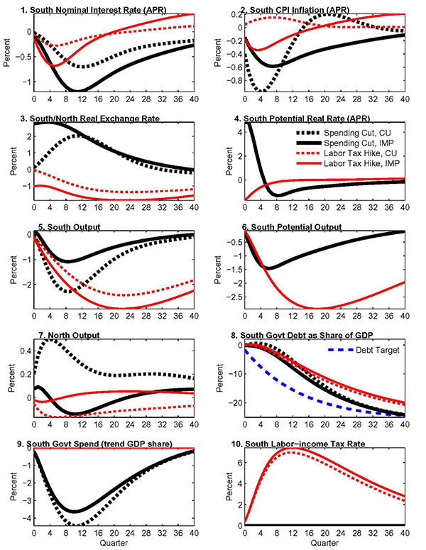
Figure 2: Baseline Scenario When Monetary Policy is Unconstrained and Subject to the Zero Lower Bound

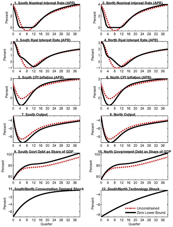
Figure 3: Debt Consolidations Via Spending Cuts and Labor-Income Tax Hikes in a 2-Year Liquidity Trap (Solid) and in Normal Times (Dotted) When South is a CU Member

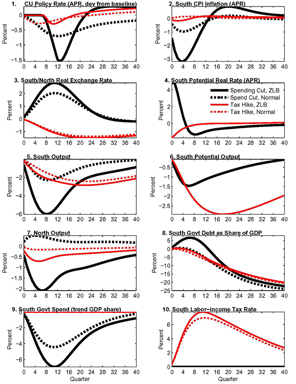
Figure 4a: Contribution to South Debt Dynamics in a Currency Union in Normal Times (When CU Mon. Pol. is Unconstrained) and in Liquidity Trap (Panel A: Spending Cuts When CU is Unconstrained)

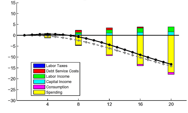
Data for Figure 4a

Quarters	Debt as share of trend GDP (sum of all bars)	Debt as share of actual GDP	Labor Taxes	Debt Service Costs	Labor Income	Capital Income	Consumption	Spending
1	0.012243	0.020451
2	-0.01944	0.252086
3	-0.13232	0.465819
4	-0.34803	0.567354	0	0.504075	0.180197	0.142859	-0.07514	-1.10002
5	-0.6785	0.510472
6	-1.12854	0.276507
7	-1.69706	-0.13635
8	-2.37792	-0.71897	0	0.971026	0.766693	0.585735	-0.23299	-4.46839
9	-3.16078	-1.45493
10	-4.03203	-2.32312
11	-4.97593	-3.29975
12	-5.97557	-4.36003	0	0.936552	1.425535	1.049073	-0.45356	-8.93318
13	-7.01386	-5.47951
14	-8.07429	-6.6351
15	-9.1416	-7.80586
16	-10.2021	-8.97341	0	0.501237	1.955606	1.376091	-0.69881	-13.3362
17	-11.2441	-10.1222
18	-12.2577	-11.2396
19	-13.2351	-12.3156
20	-14.1704	-13.3429	0	0.001	2.325444	1.555419	-0.92863	-17.0592

Figure 4b: Contribution to South Debt Dynamics in a Currency Union in Normal Times (When CU Mon. Pol. is Unconstrained) and in Liquidity Trap (Panel B: Spending Cuts When CU is in a Liquidity Trap)

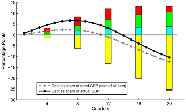
Data for Figure 4b

Quarters	Debt as share of trend GDP (sum of all bars)	Debt as share of actual GDP	Labor Taxes	Debt Service Costs	Labor Income	Capital Income	Consumption	Spending
1	0.320349	0.797601
2	0.819962	2.095629
3	1.367019	3.445241
4	1.863813	4.670711	0	1.887137	0.747955	0.560708	0.075471	-1.40746
5	2.239312	5.659401
6	2.444291	6.342602
7	2.447798	6.683768
8	2.234278	6.670694	0	4.092171	2.484777	1.78117	0.110618	-6.23446
9	1.797218	6.3063
10	1.114952	5.584098
11	0.189746	4.523556
12	-0.95799	3.165031	0	4.924763	4.321361	2.920581	-0.01211	-13.1126
13	-2.29522	1.563489
14	-3.78081	-0.21735
15	-5.32726	-2.07124
16	-6.87099	-3.91673	0	3.901303	5.742892	3.591568	-0.23542	-19.8713
17	-8.36783	-5.69635
18	-9.78892	-7.37305
19	-11.1171	-8.92587
20	-12.344	-10.3458	0	2.692413	6.751012	3.844997	-0.43278	-25.1996

Figure 5: Responses to Different Sized Debt Target Reductions in South CU Member Via Spending Cuts (Left Panels) and Labor Tax Hikes (Right Panels) in a 2-Year Liquidity Trap

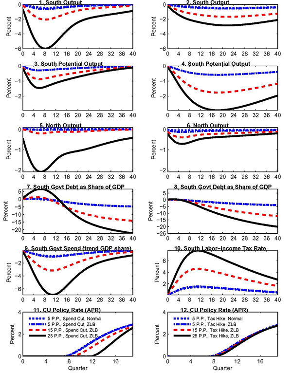
Figure 6: Marginal Output and Government Debt Multipliers in Large South to Spending Cuts and Labor Tax Hikes as Funcation of Liquidity Trap Duration

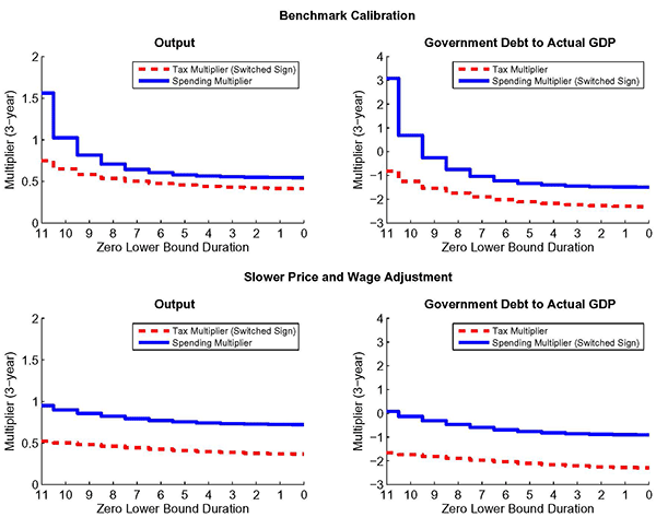
Figure 7: Pure Spending and Tax Based Debt Consolidation Strategies vs. Mix-Strategies in South CU Member in a 2-Year Liquidity Trap

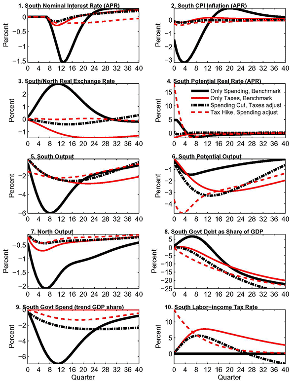
Figure 8: Sensitivity to Frisch Elasticity and Keynesian Households in South CU Member in a 2-Year Liquidity Trap: Spending Cuts (Left Panels) and Labor Tax Hikes (Right Panels)

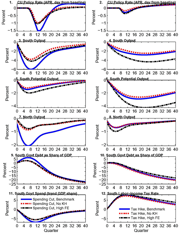
Figure 9: Sensitivity to North Response for a South Debt Target Cut of 15 P.P. in Normal Times and in a Liquidity Trap: Spending Rules (Left Panels) and Labor Tax Rules (Right Panels)

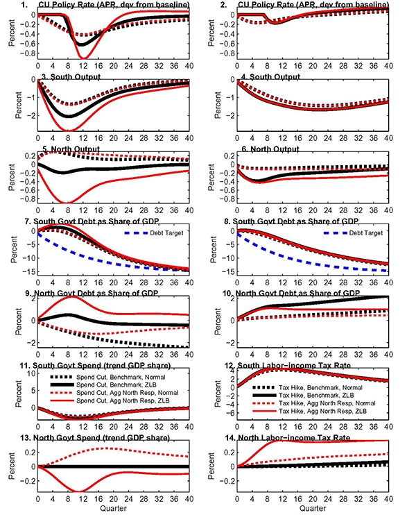
Footnotes

1.  We thank Werner Roeger and two anonymous referees for very useful comments. This paper was originally prepared for the Sveriges Riksbank conference "Monetary Policy in an Era of Fiscal Stress" (held in Stockholm June 16-17, 2011) and we thank our discussant Martin Flodén for his constructive criticism of the first draft. Moreover, our discussants Christiane Nickel (at the MONFISPOL conference at Goethe University in Frankfurt 19-20 September, 2011), Julia Lendvai (at the European Commission-Journal of Economic Dynamics and Control conference in Brussels March 2-3, 2012), Keith Kuester (at the SCIEA meeting hosted by the San Francisco Fed May 10-11, 2012), and Andrea Ferrero (at the Division of International Finance's workshop in DC, September 17-18, 2012) provided very useful comments and suggestions. Finally, we thank other conference participants, as well as seminar participants at the European Central Bank, Johns Hopkins University and the Banque de France, for helpful comments. The views expressed in this paper are solely the responsibility of the authors and should not be interpreted as reflecting the views of the Board of Governors of the Federal Reserve System or of any other person associated with the Federal Reserve System. Return to text

2.  Corresponding Author: Telephone: 202-452-3055. Fax: 202-263-4850 E-mail addresses: [email protected] and [email protected]. Return to text

3.   A normative welfare analysis of the alternative fiscal instruments would be an interesting extension, but is beyond the scope of the current analysis. Return to text

4.   Using micro-data from the Consumer Expenditure Survey, Johnson et al. (2006) and Parker et al. (2011) find evidence of a substantial response of U.S. household spending to the temporary tax rebates of 2001 and 2008. On the macro-side, Galí, López-Salio and Vallés (2007) present evidence from structural VARs that government spending shocks tend to boost private consumption, and show how the inclusion of rule-of-thumb agents in their DSGE model helps it account for this behavior. Blanchard and Perotti (2002) and Monacelli and Perotti (2008) obtain similar empirical findings. Return to text

5.   We define potential output as the level of output that would prevail if prices and wages were fully flexible. Return to text

6.   Batini et al (2012) estimate the impact of these alternative fiscal consolidation measures against the backdrop of a deep recession, and find that a tax hike has a considerably smaller contractionary effect on GDP than a similar-sized spending cut. Return to text

7.   Our result that currency union membership substantially amplifies the spending multiplier is supported by the recent empirical work of Ilzetzki, Mendoza and Vegh (2010), Serrato and Wingender (2011) and Nakamura and Steinsson (2011). Return to text

8.   We define $\xi_{t,t+j}$ to be the price in period $t$ of a claim that pays one dollar if the specified state occurs in period $t+j$ (see the household problem below); then the corresponding element of $\psi_{t,t+j}$ equals $\xi_{t,t+j}$ divided by the probability that the specified state will occur. Return to text

9.   Notice that the final investment good is not used by the government. Return to text

10.   For simplicity, we assume that $\mu_{0}$ is sufficiently small that changes in the monetary base have a negligible impact on equilibrium allocations, at least to the first-order approximation we consider. Return to text

11.   Notice that the contingent claims $B_{Dt+1}$ are in zero net supply from the standpoint of the South as a whole. Return to text

12.   Given that the central bank uses the nominal interest rate as its policy instrument, the level of seigniorage is determined by nominal money demand. Return to text

13.   Lower case letters are used to express a variable as a percent or percentage point deviation from its steady state level. Note that real government debt $b_{G,t}$ and real transfers $tr_{t}$ are defined as a share of steady state GDP and expressed as percentage point deviations from their steady state or "trend" values. That is, $b_{G,t}=\left( \frac{B_{G,t}}{P_{t}Y}\right) -b_{G}$, where $B_{G,t}$ is nominal government debt, $P_{t}$ is the price level, and $Y$ is real steady state output. Similarly, we have that $tr_{t}=\left( \frac{TR_{t}}{P_{t}Y}\right) -tr$ $.$ Return to text

14.   We follow Christiano, Motto and Rostagno (2008) by assuming that the debt contract between entrepreneurs and banks is written in nominal terms (rather than real terms as in Bernanke, Gertler and Gilchrist, 1999). For further details about the setup, see Bernanke, Gertler and Gilchrist (1999), and Christiano, Motto and Rostagno (2008). An excellent exposition is also provided in Christiano, Trabandt and Walentin (2007). Return to text

15.   In future work, it would be of interest to solve the model in a fully non-linear form. Return to text

16.   Given strategic complementarities in wage-setting, the wage markup influences the slope of the wage Phillips Curve.  Return to text

17.   As we are considering a stationary model, the debt target is eventually assumed to converge back to the steady state level $b_{G}$, but by setting $\rho_{d_{2}}=0.0001$, the convergence is very slow and irrelevant for the impact in the near- and medium term. Return to text

18.   The spending-based consolidation does keep output below potential even after ten years, in contrast to Uhlig (2010). This reflects that our consolidation scenario does not allow taxes to fall.  Return to text

19.   Note that because the shocks are assumed to be equally sized for South and North and the model calibration is symmetric (apart from the relative size of the South and North), the baseline scenario is identical for South and North. Return to text

20.   Because the results in Figure 6 are reported as deviations between the scenario with fiscal austerity measures and the baseline scenario (no austerity), the differences for the interest rate responses (reported in panel 1) can be negative once the ZLB no longer binds in the baseline scenario. Return to text

21.   Our finding that fiscal spending multipliers are augmented in a liquidity trap is consistent with the empirical VAR panel evidence provided by Corsetti, Meier and Müller (2010a), who argues that fiscal contractions have more negative effects on output in crisis periods.  Return to text

22.   Our finding that tax consolidation is contractionary with a binding ZLB differs from that of Eggertsson (2010), who argues that a tax hike could have large positive multiplier in a prolonged liquidity trap. There are several key differences between our approach which account for the seemingly disparate results. First, our model incorporates hand-to-mouth households. Second, Eggertsson considers an environment without wage stickiness. Third, Eggertsson considers front-loaded temporary hikes (for which the potential real interest rate will rise instead of fall as with our gradual tax profile). Fourth, we consider a rule-based hike (which introduces a wedge between the actual and potential labor tax rate) as opposed to an exogenous hike. Finally, we embed a higher degree of price stickiness.  Return to text

23.   This decomposition is undertaken by simulating the (log-linearized) government budget constraint (25). Notice that net transfers $TR_{t}$ are assumed to be exogenous and hence do not impact the evolution of government debt. Moreover, the steady state monetary base is assumed to be arbitrarily small, and therefore also has a neligible impact. Return to text

24.   To highlight how the duration of the liquidity trap varies with the size of fiscal consolidation, panels 11 and 12 of Figure 6 are plotted in levels, and not in deviation from baseline as in panel 1 of Figure 6.  Return to text

25.   In Figure 6, we switch the sign of $m_{K}^{debt}$ in (36) to provide a more intuitive interpretation of the debt multiplier in which either a cut in spending or rise in taxes would "normally" cause the debt/GDP ratio to fall (though the debt/GDP ratio can rise in a long-lived trap, as clear from the figure). Return to text

26.   Because of the important role of movements in inflation, it is possible that the relative merits of spending- and tax-based consolidations could be quite different in our forward-looking model under a monetary policy rule that committed the CU to price level targeting. Nevertheless, major central banks do not describe policy as oriented towards stabilizing the price level; and numerous empirical papers have shown that the policy rule we adopt (which specificies that the CU central bank responds to CU inflation rates and output gaps according to eq. 24) provides a good description of actual policy behavior. Return to text

27.   Specifically, we assume an AR(1) for the labor income tax with a root of .9. Return to text

28.   For the gradual and very persistent spending cut we specify $\Delta g_{t} =\rho_{g_{1}}\Delta g_{t-1}-\rho_{g_{2}}g_{t-1}$ and set $\rho_{g_{1}}=.75$ and $\rho_{g_{2}}=.00275.$ Return to text

29.   Specifically, we assume that the coefficients on the debt and deficit in each of the two rules are half as large as those adopted by the South, i.e. $\nu_{g_{j}}^{North}=\nu_{g_{j}}^{South}/2$ and $\nu_{\tau_{j}}^{North} =\nu_{\tau_{j}}^{South}/2$ for $j=\left\{ 1,2\right\} .$ The smoothing coefficients $\nu_{g_{0}}$ and $\nu_{\tau_{0}}$ are kept the same as in the South (i.e., at .5). Return to text

30.   The near-term effects of transfers is likely to depend on how the transfers are distributed across households. In this vein, recent research using large-scale policy models (Coenen et al., 2012) suggests that cuts in transfers that are concentrated on households facing liquidity constraints - the HM households in our setup - are likely to be associated with a larger multiplier compared to cuts to general transfers to all households. Return to text

31.   Moreover, our analysis examines fiscal consolidation in a world in which the public has complete confidence that the government will repay its nominal obligations, so that market risk premia are zero. Some recent analysis has considered the consequences of fiscal retrenchment when bond market spreads depend endogenously on government debt, including Erceg and Lindé (2010a), and Corsetti et al. (2012). Return to text

32.   As mentioned in the previous footnote, Erceg and Lindé (2010a) and Corsetti et al. (2012) has allowed for an endogenous reaction of sovereign spreads, but focused exclusively on spending-based consolidation. Return to text

This version is optimized for use by screen readers. Descriptions for all mathematical expressions are provided in LaTex format. A printable pdf version is available. Return to text

Home | Economic research and data | Publications and education resources
Accessibility | Contact us
Last update: August 29, 2013