
Board of Governors of the Federal Reserve System
International Finance Discussion Papers
Number 1078, April 2013 --- Screen Reader
Version*
A Robust Neighborhood Truncation Approach to Estimation of Integrated Quarticity
NOTE: International Finance Discussion Papers are preliminary materials circulated to stimulate discussion and critical comment. References in publications to International Finance Discussion Papers (other than an acknowledgment that the writer has had access to unpublished material) should be cleared with the author or authors. Recent IFDPs are available on the Web at http://www.federalreserve.gov/pubs/ifdp/. This paper can be downloaded without charge from the Social Science Research Network electronic library at http://www.ssrn.com/.
Abstract:
We provide a first in-depth look at robust estimation of integrated quarticity (IQ) based on high frequency data. IQ is the key ingredient enabling inference about volatility and the presence of jumps in financial time series and is thus of considerable interest in applications. We document the significant empirical challenges for IQ estimation posed by commonly encountered data imperfections and set forth three complementary approaches for improving IQ based inference. First, we show that many common deviations from the jump diffusive null can be dealt with by a novel filtering scheme that generalizes truncation of individual returns to truncation of arbitrary functionals on return blocks. Second, we propose a new family of efficient robust neighborhood truncation (RNT) estimators for integrated power variation based on order statistics of a set of unbiased local power variation estimators on a block of returns. Third, we find that ratio-based inference, originally proposed in this context by Barndorff-Nielsen and Shephard (2002), has desirable robustness properties in the face of regularly occurring data imperfections and thus is well suited for empirical applications. We confirm that the proposed filtering scheme and the RNT estimators perform well in our extensive simulation designs and in an application to the individual Dow Jones 30 stocks.
Keywords: Robust neighborhood truncation estimator, functional filtering, integrated quarticity, inference on integrated variance, inference on jumps, high-frequency data
JEL classification: C14; C15; C22; C80; G10
1 Introduction
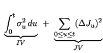
Important progress in measuring and forecasting return volatility has been obtained through techniques exploiting the information in intraday price movements. The use of high-frequency data is, however, not without its problems. The main complication is the pronounced inhomogeneity of the intraday return series as diurnal patterns interspersed with news events and market microstructure frictions complicate direct modeling of the high frequency dynamics and introduce a variety of idiosyncratic features that are largely irrelevant for inference about inter-daily volatility. The realized volatility (RV) approach "solves" this problem by aggregating the intraday return observations to a daily frequency in a manner that retains the majority of the inherent volatility information while mitigating the impact of noise and diurnal patterns. The RV approach has been widely adopted ever since its formal introduction as a nonparametric estimator of the return variation in Andersen and Bollerslev (1998).1 In parallel, a large body of theoretical work on model-free estimation and inference for components of the realized return variation process has arisen. Initial econometric issues are addressed in Andersen, Bollerslev, Diebold and Labys (2001, 2003) and Barndorff-Nielsen and Shephard (henceforth BNS) (2002).2
Conceptually, realized volatility differs from the standard notion of volatility by focusing on ex-post measurement of the realization of the (stochastic) return variation rather than the (ex-ante) return variance. Once attention shifts to the actual volatility realizations, new questions arise. For example, how do we assess the accuracy of our (daily) ex-post measures of the integrated return variation and how do we identify the impact of jump components. Such features are critical for a variety of issues in real-time financial management, including volatility forecasting, analysis of the dynamic properties of jumps and news events, derivatives pricing, estimation of return correlations, determination of return-volatility asymmetries (the leverage effect), and developing insights into the interplay between return volatility and the macroeconomic environment.
The key ingredient for inference regarding the return variation
and the presence of jumps is the so-called integrated quarticity
(IQ). To illustrate the importance of accurate IQ measures we
review a few results from the RV literature. We denote the
continuously evolving log-price for a financial asset by
![]() . Under general conditions, the log-price
constitutes a semi-martingale with respect to an underlying
filtered probability space. The associated ex-post realized
quadratic variation,
. Under general conditions, the log-price
constitutes a semi-martingale with respect to an underlying
filtered probability space. The associated ex-post realized
quadratic variation, ![]() , for
, for ![]() over
over
![]() may be decomposed into an integrated
(diffusive) volatility,
may be decomposed into an integrated
(diffusive) volatility, ![]() , and a residual (jump)
component,
, and a residual (jump)
component, ![]() ,
,
| (1) | |||
|
where ![]() and
and ![]() denote the
instantaneous drift and diffusion coefficients, while
denote the
instantaneous drift and diffusion coefficients, while ![]() and
and ![]() are adapted Wiener and finite
activity jump processes, respectively.
are adapted Wiener and finite
activity jump processes, respectively.
For a given trading day,
![]() , we consider the ideal scenario
in which we observe
, we consider the ideal scenario
in which we observe ![]() equally-spaced (log)
returns,
equally-spaced (log)
returns,
![]() ,
,
![]() . In this case, the
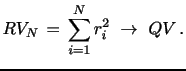
realized volatility (RV) is a consistent nonparametric estimator of
QV, as the number of intraday observations diverges,
. In this case, the
realized volatility (RV) is a consistent nonparametric estimator of
QV, as the number of intraday observations diverges,
![]() (in-fill
asymptotics),
(in-fill
asymptotics),
|
Moreover, absent price jumps, the limiting distribution is a Gaussian mixture,
where
![]() ,
which, as observed by BNS (2002), can be consistently estimated
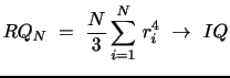
from the high-frequency data themselves via the Realized Quarticity
(RQ) statistic:
,
which, as observed by BNS (2002), can be consistently estimated
from the high-frequency data themselves via the Realized Quarticity
(RQ) statistic:
|
Clearly, accurate inference about the integrated variance hinges
on reliable estimates for IQ. Unfortunately, IQ estimation is
challenging. It involves estimating fourth order return moments
from noisy intraday return series impacted by the confounding
effects of market microstructure frictions, diurnal patterns,
outliers, and other data irregularities. For example, it is well
known that the RQ estimator is highly imprecise and non-robust to
such features, even if jumps are absent. Moreover, when discrete
price changes do occur, RV is no longer consistent for IV, and the
RQ statistic diverges:
![]() as
as
![]() . Given the
compelling evidence for jumps, this is critical in practice. In
response, various jump-robust IQ estimators have been developed,
but they are subject to potentially serious finite sample biases.
At present, there simply is no systematic evidence regarding the
performance of alternative jump-robust procedures for empirically
realistic scenarios.
. Given the
compelling evidence for jumps, this is critical in practice. In
response, various jump-robust IQ estimators have been developed,
but they are subject to potentially serious finite sample biases.
At present, there simply is no systematic evidence regarding the
performance of alternative jump-robust procedures for empirically
realistic scenarios.
Recognizing these issues, a variety of ad hoc IQ estimation procedures have been implemented in the empirical literature. Before the jump-robust theory was developed, the RQ statistic was used, but only with relatively coarse sampling. For example, BNS (2004a) exploit 10-minute foreign exchange returns, while Bandi and Russell (2008) recommend computing RQ from 15- or 20-minute returns, as sparse sampling mitigates the impact of outliers and microstructure noise. Later, BNS (2004b) and Huang and Tauchen (2005) rely on 5-minute returns for constructing jump-robust estimators of IQ.3 Finally, due to the distortions arising from market microstructure effects, Jiang and Oomen (2008) opt for simply squaring their jump-robust IV estimator to obtain an IQ estimator, thus settling for a substantial Jensen inequality bias, but aiming to reduce estimation uncertainty.
To illustrate the practical importance of jump robustness, consider drawing inference about the IV of IBM stock returns across three days in February 2008 using the non-jump robust RQ/RV measures versus a pair of jump robust measures, as shown on Figure 1.4
Figure 1: IV inference using non-jump robust RQ/RV measures versus jump-robust MedRQ/MedRV measures.
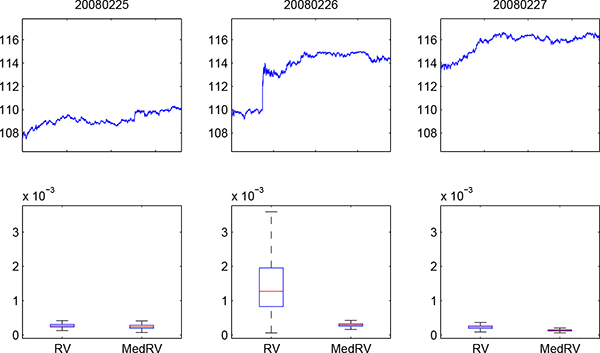
We plot prices (blue line), the IV point estimate (red line), the inter-quartile range (blue box) as well as two standard deviation IV confidence bands (black whiskers) for IBM for three trading days in February 2008.
The jump on 2/26/2008 is readily identified visually and easily detected using a jump robust test statistic. In fact, the robust MedRV estimates and associated standard error bands, based on MedRQ, suggest a relative stable volatility process across the three trading days. In contrast, the regular RV estimate for IV is greatly inflated on 2/26/2008, and the confidence band is huge, reflecting a diverging RQ statistic. Hence, the reliance on non jump-robust statistics has two consequences. First, when jumps are present the IV estimate is upward biased because the jump component in QV is attributed to IV.5 Second, the associated confidence band is grossly overstated, indicating very poor estimation precision whereas, in fact, the robust estimate appears quite reliable. Hence, non-robust inference may produce excessively erratic IV estimates and convey a sense of exaggerated imprecision associated with these techniques. While the misleading inference afforded by the regular RV and RQ estimators is apparent in Figure 1, at least when contrasted with the robust inference and a depiction of the price path, it can be less obvious in cases with higher volatility levels and relatively smaller jumps. As such, it is important to develop feasible robust and efficient procedures for estimating IQ and conducting inference for IV.
One main contribution of this paper is to provide a first
in-depth exploration of the virtues and drawbacks of alternative
jump-robust estimation procedures for IQ, including their
robustness to a variety of realistic features of the return
generating process. A point of emphasis is the use of wide
pre-averaging windows for controlling the impact of microstructure
noise on the inference. This enhances robustness and simplifies the
distribution theory as the impact of noise is annihilated
asymptotically. A second contribution is the development of a new
class of robust neighborhood truncation (RNT) estimators
that generalize existing nearest neighbor and Quantile RV
estimators. They involve the application of a second layer of order
statistics to suitably chosen return functionals, thus robustifying
the inference for IQ with only a minor loss of efficiency. We find
such RNT estimators to perform admirably, especially when used in
combination with the ratio statistic, ![]() , which
is known to provide improved finite sample inference for IV.
Moreover, these principles apply generally and can be used to
enhance the robustness of inference from alternative classes of
estimators. A third novelty is the use of an outlier filtering
procedure that operates directly on an estimation functional of
interest rather than on individual returns. This functional
filtering principle adapts the filter to the specific
assumptions underlying a given estimator. Hence, it controls the
impact, and potential distortion, of abnormal outliers within the
exact metric in which they contribute to the ultimate estimator. In
applications to individual equity return data we find this filter
indispensable for rendering entire classes of promising candidate
IQ estimators viable. The unifying theme behind our new estimators
and universal filtering procedure is to operate directly on the
functional space of local power variation estimates rather than the
individual returns. Nonetheless, the latter, and common, approach
may be obtained as a special case of our procedure.
, which
is known to provide improved finite sample inference for IV.
Moreover, these principles apply generally and can be used to
enhance the robustness of inference from alternative classes of
estimators. A third novelty is the use of an outlier filtering
procedure that operates directly on an estimation functional of
interest rather than on individual returns. This functional
filtering principle adapts the filter to the specific
assumptions underlying a given estimator. Hence, it controls the
impact, and potential distortion, of abnormal outliers within the
exact metric in which they contribute to the ultimate estimator. In
applications to individual equity return data we find this filter
indispensable for rendering entire classes of promising candidate
IQ estimators viable. The unifying theme behind our new estimators
and universal filtering procedure is to operate directly on the
functional space of local power variation estimates rather than the
individual returns. Nonetheless, the latter, and common, approach
may be obtained as a special case of our procedure.
The remainder of the paper is structured as follows. Section 2 reviews the modern approach to robust estimation of integrated power variation. Section 3 develops our robust neighborhood truncation estimators. In Section 4, we discuss additional procedures applied to obtain robustness against jumps and noise. Section 5 illustrates the importance of common data features for IQ inference through an extensive simulation study. Finally, Section 6 provides evidence using high-frequency returns on the Dow Jones 30 stocks, while Section 7 concludes. All proofs are relegated to the Appendix.
2 Overview of Jump-Robust Power Variation Estimation
This section summarizes the modern approach to power variation estimation. We outline the theoretical setting and review some existing estimators which are later used in our simulation study and empirical investigation. In the process, we discuss practical trade-offs that must be confronted in estimating objects involving high powers of volatility.
2.1 The Theoretical Setting
We focus on a single asset traded continuously in a frictionless
market over the period ![]() , referred to as a
trading day. If it is a limited-liability asset with an expected
positive payoff at some future date, the price will remain strictly
positive. No-arbitrage conditions then ensure that the log-price
process constitutes a semimartingale with respect to the underlying
filtered probability space, see, e.g., Back (1991) and Andersen,
Bollerslev and Diebold (2010). Hence, for most of our analysis we
invoke the following conditions.
, referred to as a
trading day. If it is a limited-liability asset with an expected
positive payoff at some future date, the price will remain strictly
positive. No-arbitrage conditions then ensure that the log-price
process constitutes a semimartingale with respect to the underlying
filtered probability space, see, e.g., Back (1991) and Andersen,
Bollerslev and Diebold (2010). Hence, for most of our analysis we
invoke the following conditions.
Assumption 1 The continuously compounded return
process, ![]() is governed by a jump-diffusive
semimartingale,
is governed by a jump-diffusive
semimartingale,
|
(2) |
where is![]() a locally bounded and predictable
process,
a locally bounded and predictable
process, ![]() is an adapted cadlag process bounded
away from zero, and
is an adapted cadlag process bounded
away from zero, and ![]() is a finite activity jump
process.
is a finite activity jump
process.
|
where ![]() is locally bounded and predictable,
is locally bounded and predictable,
![]() are cadlag, the
Brownian motions
are cadlag, the
Brownian motions ![]() are uncorrelated, and
are uncorrelated, and
![]() is a finite activity jump
process.
is a finite activity jump
process.
If the Brownian component in Assumption 1 is non-zero, the return innovation is an order of magnitude larger than the expected return over short time intervals, implying that the drift term typically does not affect the asymptotic distribution of power variation estimators based on high-frequency data. Hence, we ignore the drift term in this section.6
Another key implication of Assumptions 1 and 1A is that we may
derive the asymptotic properties of many relevant estimators
assuming that the intraday returns are locally Gaussian. To
operationalize this approach, the trading period is broken into
![]() smaller blocks. For each block, we treat
volatility as constant, even if the actual return variation evolves
stochastically and the price path contains finite activity jumps.
If
smaller blocks. For each block, we treat
volatility as constant, even if the actual return variation evolves
stochastically and the price path contains finite activity jumps.
If ![]() equally-spaced continuously compounded
returns are available, and each block contains
equally-spaced continuously compounded
returns are available, and each block contains ![]() returns, we assume, without loss of generality, that
returns, we assume, without loss of generality, that
![]() . Notice that each block covers
. Notice that each block covers
![]() of the trading
period and each return reflects the price evolution over an
interval length of
of the trading
period and each return reflects the price evolution over an
interval length of
![]() .
.
The above insight simplifies matters greatly, as nonparametric
jump-robust estimators now are easy to devise. One simply selects a
suitable unbiased estimator for the (power of) volatility within
each block under the null hypothesis of i.i.d. Gaussian returns,
and then cumulate the estimates across blocks to obtain the overall
power variation. The distribution theory is developed using
standard in-fill asymptotics, letting ![]() grow
indefinitely, while requiring
grow
indefinitely, while requiring
![]() . In most cases,
. In most cases,
![]() is fixed and
is fixed and ![]() diverges
proportionally with
diverges
proportionally with ![]() .
.
2.2 Estimating Power Variation under the Diffusive Null Hypothesis
We first consider the case where there is no jump component.
Given the assumptions invoked above, we focus on the null
hypothesis that the returns within a small block are i.i.d.
Gaussian. A generic estimator of the
![]() order return variation, for
order return variation, for
![]() an even positive integer, is now obtained
as the average of local estimates of
an even positive integer, is now obtained
as the average of local estimates of
![]() based on a functional
based on a functional
![]() operating on blocks of
operating on blocks of ![]() adjacent returns. For each integer
adjacent returns. For each integer
![]() , we have a return
block,
, we have a return
block,
![]() . Under the null, these returns are i.i.d.
. Under the null, these returns are i.i.d.
![]() . We
let
. We
let
![]() denote the
functional exploited by a given estimator to obtain an unbiased
estimate of
denote the
functional exploited by a given estimator to obtain an unbiased
estimate of
![]() for the
for the ![]() 'th block. If Assumption 1 holds, the power variation
estimator is consistent. Heuristically, the law of large numbers
implies, as
'th block. If Assumption 1 holds, the power variation
estimator is consistent. Heuristically, the law of large numbers
implies, as
![]() ,
,
|
A corresponding central limit theory may typically be devised if we invoke Assumption 1A.
The simplest estimator within this framework is the realized
Power Variation (PV) measure. It does not exploit multi-return
blocks, so ![]() . It takes the form,
. It takes the form,
The normalization constant is given by
![]() , for any
, for any ![]() .
.
For ![]() , this produces the regular RV, or
PV
, this produces the regular RV, or
PV![]() (2), estimator with
(2), estimator with ![]() ,
while
,
while ![]() yields the RQ, or PV
yields the RQ, or PV![]() (4), estimator from Section 1 with normalizing constant
(4), estimator from Section 1 with normalizing constant
![]() .
.
A couple of comments are warranted. First, the setting ignores
data errors and market microstructure frictions. Higher order
return moments are particularly sensitive to faulty price
observations or inappropriate assumptions regarding the evolution
of the high frequency returns. We discuss these issues in the
context of the simulation and empirical sections below. Second, in
contrast to the realized power variation estimator, the functional
![]() will in the following be designed to be
jump-robust, i.e., provide valid asymptotic inference for the power
variation, even in the presence of finite activity jumps. However,
jumps often have a severe adverse effect on the finite sample
properties of the estimators, especially for
will in the following be designed to be
jump-robust, i.e., provide valid asymptotic inference for the power
variation, even in the presence of finite activity jumps. However,
jumps often have a severe adverse effect on the finite sample
properties of the estimators, especially for ![]() . Many of the practical complications below arise
from this feature.
. Many of the practical complications below arise
from this feature.
2.3 Jump-Robust Power Variation Estimation
We now outline the basic principles behind the construction of
power variation estimators that are robust to the presence of
finite activity jump processes. Asymptotically, as the block sizes
shrink towards zero and the number of blocks grows indefinitely,
there will be a finite number of blocks containing one single jump
each. Hence, in the limit, the power variation associated with the
blocks containing jumps is negligible. It follows that the power
variation can be estimated consistently as long as the contribution
from the "jump blocks" is an order of magnitude less than the
overall power variation measure which, of course, is ![]() . However, the jumps are also of order
. However, the jumps are also of order ![]() , so the functional
, so the functional ![]() must ensure that
the jumps are dampened sufficiently to eliminate their impact
asymptotically.
must ensure that
the jumps are dampened sufficiently to eliminate their impact
asymptotically.
Formally, for any given sampling frequency, we denote the set of
indices corresponding to returns for which the associated block
contains a jump by ![]() . Thus, for
. Thus, for ![]() , there is a jump in the return block
, there is a jump in the return block
![]() . We then write the
generic power variation estimator as,
. We then write the
generic power variation estimator as,
|
The first term estimates the integrated power variation consistently, i.e.,
 as
as |
The contribution from the blocks containing jumps is negligible,
in the limit, only if each such block is of order less than
![]() . Thus, the associated power variation
estimator is consistent as long as
. Thus, the associated power variation
estimator is consistent as long as
![]() for
for
![]() .7. This is accomplished
in different ways by alternative jump-robust estimators. Moreover,
their practical effectiveness is largely determined by the degree
to which they accomplish sufficient dampening of the jump
contributions in finite samples.
.7. This is accomplished
in different ways by alternative jump-robust estimators. Moreover,
their practical effectiveness is largely determined by the degree
to which they accomplish sufficient dampening of the jump
contributions in finite samples.
2.4 Alternative Jump-Robust Power Variation Estimators
2.4.1 Multi-Power Variation Estimators
The first (finite activity) jump-robust power variation estimators were the Realized Multi-Power Variation (MPV) statistics, inspired by BNS (2002). Expressed in terms of the functional applied to successive return blocks, the estimator takes the form,
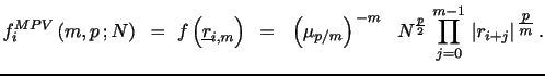
|
For ![]() and
and ![]() or
or ![]() , the estimator reduces to the (non jump-robust) RV or RQ
estimator, respectively. Prominent (jump robust) special cases
include
, the estimator reduces to the (non jump-robust) RV or RQ
estimator, respectively. Prominent (jump robust) special cases
include
![]() , which defines the bipower
variation statistic, and various IQ estimators, such as tripower
, which defines the bipower
variation statistic, and various IQ estimators, such as tripower
![]() , quadpower
, quadpower
![]() , and quintpower
, and quintpower
![]() .
.
As described earlier, the actual estimator is now obtained by averaging the value of the functional across the available blocks,
|
The MPV estimator is consistent and affords an associated CLT,
as long as ![]() is chosen sufficiently large relative
to
is chosen sufficiently large relative
to ![]() . This produces an inevitable bias-variance
trade-off. A larger
. This produces an inevitable bias-variance
trade-off. A larger ![]() implies more dampening of
the jump term, so the finite sample bias induced by the jump is
alleviated. On the other hand, for a given sampling frequency, a
larger block size,
implies more dampening of
the jump term, so the finite sample bias induced by the jump is
alleviated. On the other hand, for a given sampling frequency, a
larger block size, ![]() , implies that the
functional is less localized, so the constant volatility assumption
provides a poorer approximation, and the estimator becomes less
efficient.
, implies that the
functional is less localized, so the constant volatility assumption
provides a poorer approximation, and the estimator becomes less
efficient.
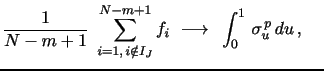
2.4.2 Truncated Power Variation Estimators
An estimator closely related to the PV and MPV statistics is the
Realized Truncated Power Variation (TPV) measure. Mancini (2009)
introduces the threshold realized volatility and quarticity
estimators, while Corsi, Pirino and Reno (2010), henceforth CPR,
consider a bipower variant of these statistics. These estimators
achieve jump robustness by truncating observations exceeding a
pre-specified threshold. Under in-fill asymptotics, we may
stipulate that the threshold converges toward zero slowly enough
(slower than
![]() ) that the limiting
distribution of the resulting estimators is identical to their
non-truncated counterparts. In particular, Truncated RV, or TRV, is
asymptotically most efficient among all jump robust IV estimators,
and similarly the Truncated RQ, or TRQ, is the most efficient
jump-robust estimator for IQ. Moreover, it is evident that the
(finite sample) jump distortion is determined by the size of the
truncation threshold and thus is under direct control in designing
the estimator. The block-functional defining the truncation
multi-power variation estimator of order
) that the limiting
distribution of the resulting estimators is identical to their
non-truncated counterparts. In particular, Truncated RV, or TRV, is
asymptotically most efficient among all jump robust IV estimators,
and similarly the Truncated RQ, or TRQ, is the most efficient
jump-robust estimator for IQ. Moreover, it is evident that the
(finite sample) jump distortion is determined by the size of the
truncation threshold and thus is under direct control in designing
the estimator. The block-functional defining the truncation
multi-power variation estimator of order ![]() with
truncation threshold,
with
truncation threshold,
![]() , takes the
form,
, takes the
form,
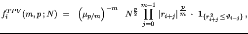
|
where
![]() is an indicator function,
taking the value of one if the statement A is true, and zero
otherwise. As before, the actual TPV
is an indicator function,
taking the value of one if the statement A is true, and zero
otherwise. As before, the actual TPV![]() (m,p)
estimator is obtained by averaging the functional values across the
available return blocks for the trading period.
(m,p)
estimator is obtained by averaging the functional values across the
available return blocks for the trading period.
The choice of threshold can be delicate. It is beneficial to
truncate aggressively to reduce the jump distortion by choosing a
low threshold, but the non-jump returns are then also truncated
with non-trivial probability. CPR suggest a finite-sample scaling
to correct for this bias. They develop an iterative scheme aiming
to obtain a fixed point at which the expectation of the truncated
estimator equals the true (estimated) volatility under the null
hypothesis. The approach is conceptually appealing, but has
drawbacks. First, the modified estimator is no longer linear in the
unobserved
![]() and thus suffers from a downwards
bias, due to Jensen's inequality, even in the ideal Brownian case.
Second, they use a sizeable two-sided window (e.g., 50
observations) to obtain a local volatility estimate, thereby
rendering it susceptible to an additional bias due to time
variation in volatility across the block.
and thus suffers from a downwards
bias, due to Jensen's inequality, even in the ideal Brownian case.
Second, they use a sizeable two-sided window (e.g., 50
observations) to obtain a local volatility estimate, thereby
rendering it susceptible to an additional bias due to time
variation in volatility across the block.
2.4.3 Neighborhood Truncation Estimators
Andersen, Dobrev and Schaumburg, henceforth ADS, (2012) introduce a couple of IV estimators, MinRV and MedRV, designed to improve on the trade-off between jump robustness and efficiency confronting the MPV estimators. MinRV and MedRV are based on an endogenous "nearest neighbor" truncation which is particularly helpful in alleviating the finite-sample impact of isolated large jumps. We now extend this theory to cover general power variation estimation. We start out by introducing notation that allows us to identify various order statistics associated with a given return block.
First, we denote the
![]() th block, consisting of absolute returns
raised to the
th block, consisting of absolute returns
raised to the
![]() power, by
power, by
![]() Next,
Next,
![]() indicates the
indicates the
![]() order statistic of the block
order statistic of the block
![]() , so
, so
![]() . As the returns are assumed
. As the returns are assumed
![]() we may
also write
we may
also write
![]() , highlighting the fact that all estimators for the block
ultimately are functionals operating on the realization of an
, highlighting the fact that all estimators for the block
ultimately are functionals operating on the realization of an
![]() -dimensional standard normal random
vector.
-dimensional standard normal random
vector.
We now readily obtain ![]() separate unbiased
estimators for
separate unbiased
estimators for
![]() , namely one for each order
statistic. We denote these "Neighborhood Truncation" estimators,
or NT
, namely one for each order
statistic. We denote these "Neighborhood Truncation" estimators,
or NT![]() (j,m,p). As before, we construct them by
averaging the appropriate block functional across the trading
period. The functional takes the form,
(j,m,p). As before, we construct them by
averaging the appropriate block functional across the trading
period. The functional takes the form,
|
where
![]() This normalization ensures that the functional provides an
unbiased estimator for
This normalization ensures that the functional provides an
unbiased estimator for
![]() . Since the scaling factors
are inversely related to the expected value of the order
statistics, we have the ranking,
. Since the scaling factors
are inversely related to the expected value of the order
statistics, we have the ranking,
![]() . For
high values of
. For
high values of ![]() and
and ![]() , these
factors become quite large for the lower order statistics, while
they are very small for the higher order statistics.8
, these
factors become quite large for the lower order statistics, while
they are very small for the higher order statistics.8
The class of neighborhood truncation estimators generalize the
MinRV and MedRV estimators, as we have,
![]() and
and
![]() .9 Under appropriate
conditions the NT estimators are consistent and afford a CLT. We
confirm this result when we introduce an even wider class of robust
estimators in Section 3.
.9 Under appropriate
conditions the NT estimators are consistent and afford a CLT. We
confirm this result when we introduce an even wider class of robust
estimators in Section 3.
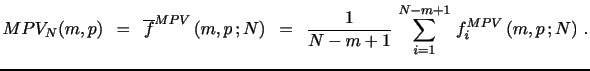
2.4.4 Combining Power Variation Estimators
It seems natural to combine some of the estimators introduced above to obtain superior asymptotic properties and, possibly, improved finite-sample performance. It is, however, outside the scope of the current paper to pursue this topic in depth. Nonetheless, we do develop the framework and notation to accommodate such combination estimators, as it is useful for our introduction of a new class of robust estimators in the next section.
Assume we have a candidate set of ![]() separate
jump-robust power variation estimators which all are unbiased,
consistent and afford a CLT under the local Gaussian null
hypothesis. We denote this set of estimators,
separate
jump-robust power variation estimators which all are unbiased,
consistent and afford a CLT under the local Gaussian null
hypothesis. We denote this set of estimators,
![]() Almost trivially, it is then, in theory, feasible to improve the
performance of any single estimator by combining it with
others.10
Almost trivially, it is then, in theory, feasible to improve the
performance of any single estimator by combining it with
others.10
We formalize the selection of a subset of the estimators by
introducing a "selection" vector, identifying the elements in
![]() used to construct a given
(combination) estimator. Hence, we let the
used to construct a given
(combination) estimator. Hence, we let the ![]() x
x![]() vector
vector
![]() consisting of an ordered subset of integers from
consisting of an ordered subset of integers from
![]() indicate
that the combination estimator is based on the set
indicate
that the combination estimator is based on the set
![]() . Denoting the set of all possible selector vectors
. Denoting the set of all possible selector vectors
![]() , any subset is now uniquely
identified by
, any subset is now uniquely
identified by
![]() , where
, where
![]() ranges from a scalar
(using a single estimator), at the one extreme, to the full vector
ranges from a scalar
(using a single estimator), at the one extreme, to the full vector
![]() (using them
all), at the other extreme.
(using them
all), at the other extreme.
A natural way to preserve the desirable properties of the
individual estimators is to exploit linear combinations with
non-negative weights that sum to unity. For example, focusing
exclusively on a set of NT estimators constructed using a return
block of size ![]() , we have
, we have
![]() , where each element represents an unbiased estimator based on the
corresponding (absolute return) order statistic. Picking a specific
NT estimator amounts to, a priori, selecting a given integer
, where each element represents an unbiased estimator based on the
corresponding (absolute return) order statistic. Picking a specific
NT estimator amounts to, a priori, selecting a given integer
![]() There
are a total of
There
are a total of ![]() distinct non-empty subsets
of
distinct non-empty subsets
of
![]() from which to construct a
combination estimator. It is a routine exercise to extend our
asymptotic results to cover the case of any such linear combination
of NT estimators.11 Conceptually, it is likewise
straightforward to derive corresponding results for linear
combinations involving alternative types of jump-robust
estimators.
from which to construct a
combination estimator. It is a routine exercise to extend our
asymptotic results to cover the case of any such linear combination
of NT estimators.11 Conceptually, it is likewise
straightforward to derive corresponding results for linear
combinations involving alternative types of jump-robust
estimators.
In summary, within the ideal setting of Assumptions 1 and 1A, superior asymptotic performance can be obtained by combining the information associated with all available estimators. However, this must be weighed against the robustness objective of ensuring reliable finite sample inference in the presence of jumps as well as other potential sources of noise. Such robustness concerns motivate the introduction of an even broader class of combination estimators in the following section, obtained by nonlinearly combining suitably chosen unbiased estimators via a second layer of order statistics.
3 Robust Neighborhood Truncation Estimation
Our major objective is to develop a reliable jump-robust procedure for estimating measures associated with the integrated quarticity. Most of the estimators reviewed in the previous section were developed for IV, even if they can be adapted for higher order power variation measures. It is worth recognizing that the relative importance of factors impacting the trade-off between statistical efficiency and robustness changes substantially as we estimate higher order power variation measures. In fact, our simulation evidence demonstrates, quite strikingly, that the most suitable approach for IV estimation is unlikely to be preferable when estimating IQ. Consequently, we now introduce a novel inference procedure which enhances the robustness to common sources of finite-sample distortions and allows for a great deal of flexibility in implementation so that the estimator can be tailored to the specific features of a given return series and market environment.
3.1 Theory
This section proposes estimating integrated power variation via a nonlinear combination of existing unbiased estimators, obtained by invoking an additional layer of order statistics. We develop the theory for neighborhood truncation estimators, but the principles apply for any set of unbiased estimators. The emphasis is on finite sample robustness to microstructure noise and jumps, so we label them "Robust Neighborhood Truncation," or RNT, estimators.
For a return block of size ![]() , there are
, there are
![]() distinct NT estimators, namely one for
each order statistic. One may combine any subset of these to
produce an estimator that exploits more sampling information than
can be utilized by any individual one. The set of alternative
selections is the set,
distinct NT estimators, namely one for
each order statistic. One may combine any subset of these to
produce an estimator that exploits more sampling information than
can be utilized by any individual one. The set of alternative
selections is the set,
![]() , of non-empty subsets of
, of non-empty subsets of
![]() . A specific
choice is given by
. A specific
choice is given by
![]() The corresponding NT estimators are defined via the functionals
they apply to the underlying return blocks. To facilitate the
exposition, we use the following short-hand notation for these
functionals, applied to the
The corresponding NT estimators are defined via the functionals
they apply to the underlying return blocks. To facilitate the
exposition, we use the following short-hand notation for these
functionals, applied to the
![]() return block,
return block,
The rationale behind the NT estimators is to alleviate the
impact of extreme returns - large or small - which may be
incompatible with the i.i.d. Gaussian assumption. The robust
neighborhood truncation principle takes the reasoning one step
further by producing an estimator for
![]() based on a suitable order
statistic among the subset of selected NT estimators. Formally, we
have,
based on a suitable order
statistic among the subset of selected NT estimators. Formally, we
have,

|
where
![]()
Normalization is required, even if each NT estimator is
individually unbiased, because selection conditional on
observed realizations induces a bias. This is corrected by scaling
with (the inverse of) the expected value of the corresponding order
statistic for a standard normal ![]() x
x![]() vector. This normalization factor is not available in closed form,
but may be determined, to any degree of accuracy, by numerical
integration or simulation.
vector. This normalization factor is not available in closed form,
but may be determined, to any degree of accuracy, by numerical
integration or simulation.
As before, the actual estimator is obtained by averaging the estimates across all blocks in the trading periods, so we have,
|
Notice that the RNT procedure involves two layers of order
statistics: we first construct consistent NT estimators from the
order statistics of a block of absolute returns (which readily may
be extended to any set of consistent estimators), and then obtain
the RNT estimator from another order statistic applied to a subset
of these NT estimators. This provides a great deal of flexibility
in alleviating the impact of extreme returns. In line with the
logic behind the MinRV and MedRV measures, the RNT estimator is
consistent if we exclude the largest order statistic from
![]() . Asymptotically, this ensures that
none of the NT estimators are generated from a (scaled) jump
return. Alternatively, this is also guaranteed if we avoid
constructing the RNT estimator from the largest realization of the
NT estimators, i.e.,
. Asymptotically, this ensures that
none of the NT estimators are generated from a (scaled) jump
return. Alternatively, this is also guaranteed if we avoid
constructing the RNT estimator from the largest realization of the
NT estimators, i.e., ![]() in the second
step.
in the second
step.
Proposition 1 Let a family of ![]() distinct NT estimators,
indexed by
distinct NT estimators,
indexed by ![]() , be generated from absolute
return blocks of size
, be generated from absolute
return blocks of size ![]() . The largest order
statistic used for constructing any of these NT estimators is
denoted
. The largest order
statistic used for constructing any of these NT estimators is
denoted ![]() ,
,
![]() . Next, consider the RNT estimator
obtained from the
. Next, consider the RNT estimator
obtained from the
![]() order statistic app
order statistic app![]() lied to
this family of NT estimators,
lied to
this family of NT estimators, ![]()
![]() .
.
If (i) Assumption 1 holds; (ii)
and/or ; and (iii) ![]() is a positive, even integer; then, as
is a positive, even integer; then, as
![]()
|
If, in addition, Assumptions 1A applies, we obtain, for
![]() a known
constant,
a known
constant,

|
The proposition warrants a few comments. First, the distributional
convergence is stable with a mixed Gaussian limit, i.e., a normal
distribution conditional on the realization of the integrated power
variation,
![]() ,
where, importantly, the limiting normal variate is independent of
the (random) power variation process.12 Second, the
convergence result is qualitatively similar to those established
for existing power variation estimators, with the "efficiency
factor"
,
where, importantly, the limiting normal variate is independent of
the (random) power variation process.12 Second, the
convergence result is qualitatively similar to those established
for existing power variation estimators, with the "efficiency
factor"
![]() determining the
relative asymptotic efficiency of the estimator. Third, the main
objective is not efficiency per se, but good performance along with
(finite sample) robustness to jumps, noise, and other data
irregularities. Fourth, the results apply for the Neighborhood
Truncation and Nearest Neighbor Truncation estimators, as these
constitute special cases involving a particular choice for the
vector I. Fifth, the results are likely to extend to
the infinite activity jump case, given suitably tight constraint on
the size of the associated (jump) activity index.13
determining the
relative asymptotic efficiency of the estimator. Third, the main
objective is not efficiency per se, but good performance along with
(finite sample) robustness to jumps, noise, and other data
irregularities. Fourth, the results apply for the Neighborhood
Truncation and Nearest Neighbor Truncation estimators, as these
constitute special cases involving a particular choice for the
vector I. Fifth, the results are likely to extend to
the infinite activity jump case, given suitably tight constraint on
the size of the associated (jump) activity index.13
3.2 Illustration
The simulation and empirical work in the following sections
exploit fairly small blocks of ![]() in order to
retain resiliency relative to rapidly changing volatility levels
during the trading day. In addition, we find it useful to eliminate
estimators that stem from the lowest order statistics of the
absolute returns as these are relatively more affected by market
microstructure noise such as price discreteness and bid-ask bounce.
This is a particular concern, because these estimates are
bias-corrected by scaling the original small returns by a large
factor, implying that microstructure distortions may be amplified.
Likewise, we typically satisfy the formal constraint on the order
statistics by picking
in order to
retain resiliency relative to rapidly changing volatility levels
during the trading day. In addition, we find it useful to eliminate
estimators that stem from the lowest order statistics of the
absolute returns as these are relatively more affected by market
microstructure noise such as price discreteness and bid-ask bounce.
This is a particular concern, because these estimates are
bias-corrected by scaling the original small returns by a large
factor, implying that microstructure distortions may be amplified.
Likewise, we typically satisfy the formal constraint on the order
statistics by picking ![]() , so we avoid basing
the RNT estimator on the largest realization among the relevant NT
estimators.
, so we avoid basing
the RNT estimator on the largest realization among the relevant NT
estimators.
For a ![]() -dimensional return block, the construction
of the
-dimensional return block, the construction
of the
![]() and
and
![]() estimators
are exemplified in Figure 2. The
notation becomes quite involved so, for brevity, we refer to the
two estimators in the diagram as and , respectively.14 Both
play a significant role in our subsequent exposition. For these
estimators, the two smallest absolute returns are discarded, while
the remaining three are used to compute the corresponding NT
estimators. Among those, we pick the lowest, respectively median,
realization and scale it to construct the associated RNT
estimator.
estimators
are exemplified in Figure 2. The
notation becomes quite involved so, for brevity, we refer to the
two estimators in the diagram as and , respectively.14 Both
play a significant role in our subsequent exposition. For these
estimators, the two smallest absolute returns are discarded, while
the remaining three are used to compute the corresponding NT
estimators. Among those, we pick the lowest, respectively median,
realization and scale it to construct the associated RNT
estimator.
Figure 2: Schematic representation of the construction of the and
estimators of
![]() on a block of five adjacent
returns.
on a block of five adjacent
returns.
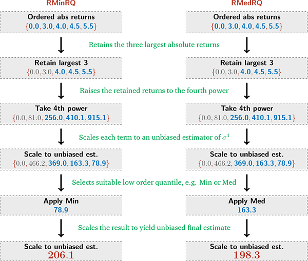
A few features are worth emphasizing. First, we display the NT
estimators obtained from the first two order statistics along with
the rest, even if they are excluded from the construction of the
estimator. Hence, the third box displays all five returns taken to
the fourth power. An extreme right skew is evident, with values
spanning 0 to 915.1, even if the initial returns are not
particularly scattered. A zero return is, of course, common due to
the discreteness of the price grid. Second, between box 3 and 4 we
apply the relevant scaling factors for the NT estimators, see Panel
B of Table 1. Strikingly, the
large factor (5.74 = (0.1741)![]() ) for the
second order statistic produces, by far, the largest realized
estimator in box 4 (466.2). Finally, excluding the NT estimators
originating from the two smallest absolute returns (0, 466.2), we
pick the minimum and median of the remainder and scale these
statistics (78.9 and 163.3) suitably with the scaling factors
provided in Panel D of Table 1 (2.611 =
(0.38303)
) for the
second order statistic produces, by far, the largest realized
estimator in box 4 (466.2). Finally, excluding the NT estimators
originating from the two smallest absolute returns (0, 466.2), we
pick the minimum and median of the remainder and scale these
statistics (78.9 and 163.3) suitably with the scaling factors
provided in Panel D of Table 1 (2.611 =
(0.38303)![]() and 1.214 = (0.82367)
and 1.214 = (0.82367)![]() ) to obtain the local RNT estimators for
) to obtain the local RNT estimators for
![]() of 206.1 given by ,
respectively 198.3 given by . These realizations happen to stem
from the two largest order statistic of the original return block
(5.5 and 4.5), but the low scaling factors for these order
statistics (0.086 = (11.59249)
of 206.1 given by ,
respectively 198.3 given by . These realizations happen to stem
from the two largest order statistic of the original return block
(5.5 and 4.5), but the low scaling factors for these order
statistics (0.086 = (11.59249)![]() and 0.398 =
(2.51102)
and 0.398 =
(2.51102)![]() ) imply that the associated (unbiased)
NT estimators in box 4 are the smallest among the relevant subset.
It reflects the relatively low spread between the three largest
absolute return realizations of 4.0, 4.5, and 5.5. In general,
these procedures tend to moderate the local estimates relative to
estimators which rely more directly on the raw fourth powers in box
3.
) imply that the associated (unbiased)
NT estimators in box 4 are the smallest among the relevant subset.
It reflects the relatively low spread between the three largest
absolute return realizations of 4.0, 4.5, and 5.5. In general,
these procedures tend to moderate the local estimates relative to
estimators which rely more directly on the raw fourth powers in box
3.
Table 1a: Tabulation of Moments of Order Statistics for Standard Gaussian Return Blocks of up to Five Returns - Panel A: 2nd Moments Defining the Inverse Scaling Factors for Corresponding NTV Estimators
| Block Size | Z2(1) | Z2(2) | Z2(3) | Z2(4) | Z2(5) |
|---|---|---|---|---|---|
| 2 | µ2(1,2) ≈1.6366198 =π - 2/π | µ2(2,2) ≈0.36338023 =2 + π/π | |||
| 3 | µ2(1,3) ≈0.19279847 =-6+2√3+π/π | µ2(2,3) ≈0.70454374 =6-4√3+π/π | µ2(3,3) ≈ 2.1026578 =1+2√3/π | ||
| 4 | µ2(1,4) ≈0.12070214 =1+4(4√3-9)/3π | µ2(2,4) ≈0.40908747 =12-8√3+π/π | µ2(3,4) ≈1 | µ2(4,4) ≈2.4702104 = 1 + 8/ √ 3π | |
| 5 | µ2(1,5)≈0.083077313 | µ2(2,5)≈0.271201456 | µ2(3,5)≈0.61591649 | µ2(4,5)≈1.2560557 | µ2(5,5)≈2.7737491 |
Table 1b: Tabulation of Moments of Order Statistics for Standard Gaussian Return Blocks of up to Five Returns - Panel B: 4th Moments Defining the Inverse Scaling Factors for Corresponding NTQ Estimators
| Block Size | Z4(1) | Z4(2) | Z4(3) | Z4(4) | Z4(5) |
|---|---|---|---|---|---|
| 2 | µ4(1,2)≈0.45352091 =3-8/π | µ4(2,2)≈5.5464791 =3+8/π | |||
| 3 | µ4(1,3)≈0.13874649 =3+26-24√3/√3π | µ4(2,3)≈1.0830697 =72-52√3+9π/3π | µ4(3,3)≈7.7781838 =3+26/√3π | ||
| 4 | µ4(1,4)≈ 0.057664089 =3+4(4(13√3-27)π-9/9π2 | µ4(2,4)≈0.38199370 =3+4(9+(36-26√3)π)//3π2 | µ4(3,4)≈1.7841458 =3-12/π2 | µ4(4,4)≈9.7761964 =3+4(9+26√3π)/9π2 | |
| 5 | µ4(1,5)≈0.028554808 | µ4(2,5)≈0.17410122 | µ4(3,5)≈0.69383242 | µ4(4,5)≈2.5110214 | µ4(5,5)≈11.592490 |
Table 1c: Tabulation of Moments of Order Statistics for Standard Gaussian Return Blocks of up to Five Returns - Panel C: 2nd Moments Defining the Inverse Scaling Factors for Corresponding RNTV Estimators
| Block Size | min( Z2(3) / µ2(3,5) ,Z2(4) / µ2(4,5) ,Z2(5) / µ2(5,5) ) | med( Z2(3) / µ2(3,5) ,Z2(4) / µ2(4,5) ,Z2(5) / µ2(5,5) ) |
|---|---|---|
| 5 | µ2(1,(3,4,5)) ≈0.62084 | µ2(2,(3,4,5)) ≈ 0.94544 |
Table 1d: Tabulation of Moments of Order Statistics for Standard Gaussian Return Blocks of up to Five Returns - Panel D: 4th Moments Defining the Inverse Scaling Factors for Corresponding RNTQ Estimators
| Block Size | min( Z4(3) / µ4(3,5) ,Z4(4) / µ4(4,5) ,Z4(5) / µ4(5,5) ) | med( Z4(3) / µ4(3,5) ,Z4(4) / µ4(4,5) ,Z4(5) / µ4(5,5) ) |
|---|---|---|
| 5 | µ4(1,(3,4,5)) ≈0.38303 | µ4(2,(3,4,5)) ≈ 0.82367 |
We compute the second and fourth moments of order statistics based on blocks of powers of independent standard normals, Zi~N(0, 1), whose inverse represent the scaling factors of the NT and RNT estimators defined in sections 2.4.3 and 3.1. Panel A: Expectation of order statistics of squared normals (NTV estimators). Panel B: Expectation of order statistics of normals raised to the 4th power (NTQ estimators). Panel C: Expectation of quantiles of rescaled squared order statistics of normals (RNTV estimators). Panel D: Expectation of quantiles of rescaled order statistics of normals raised to the 4th power (RNTQ estimators).
4 Robustification Towards Noise and Errors
In estimating higher order return power variation measures, we
deal with procedures that can be highly sensitive to erroneous
outliers as well as the presence of noise. Hence, we adopt various
techniques that mitigate the impact of such features on the
inference. Our strategy includes standard pre-filtering for obvious
data errors, pre-averaging to reduce the magnitude of the noise in
the returns, and conducting inference on the ratio of ![]() versus
versus ![]() rather than directly for
rather than directly for
![]() . However, most inference techniques
continue to display excessive sensitivity to data irregularities.
Consequently, we supplement the above steps with a novel filtering
method, specifically designed for robust power variation estimators
operating on return blocks. This section reviews the techniques we
employ to enhance the robustness of our inference towards data
errors and noise.
. However, most inference techniques
continue to display excessive sensitivity to data irregularities.
Consequently, we supplement the above steps with a novel filtering
method, specifically designed for robust power variation estimators
operating on return blocks. This section reviews the techniques we
employ to enhance the robustness of our inference towards data
errors and noise.
4.1 Eliminating Obvious Errors in the Tick-by-Tick Data
Any large set of raw transactions data is invariably subject to recording errors that infuse noise into the high-frequency returns. Most dramatically, faulty prices create artificial outliers, causing so-called "bounce-backs" in returns, as there is a "jump" both when the flawed price first appears and later, often shortly thereafter, when the price reverts to the correct level. Hence, the need for effective cleaning procedures has long been acknowledged. BNHLS (2009) lay out a systematic framework for dealing with trade data from NYSE-TAQ. In their terminology, we apply the filters P1-P3 and T1-T4.15 These filters are arguably mild and uncontroversial and simply aim to eliminate obvious data errors.
4.2 Pre-Averaging
The assumption that (observed) high-frequency returns embody a
diffusive component is systematically violated at the tick-by-tick
level due to various market microstructure features, including the
finite price grid and the bid-ask spread. As a result, tick-by-tick
price changes are often an order of magnitude larger than what is
consistent with a diffusive characterization. One effective
approach to mitigating the impact of such noise is to apply
pre-averaging, as originally suggested by Podolskij and Vetter
(2009a). This is achieved by transforming the noisy observations on
ultra high-frequency returns into a smaller set of kernel-averaged,
and thus less erratic, "smoothed" returns. In particular, each of
the ![]() returns within a block are obtained via
kernel-averaging based on separate, non-overlapping subsets of
tick-by-tick returns. The benefit is a reduction in the impact of
idiosyncratic noise and, especially, distortions induced by
bounce-backs. The drawback is a substantial drop in the underlying
sampling frequency. The latter impacts the choice of the window
width,
returns within a block are obtained via
kernel-averaging based on separate, non-overlapping subsets of
tick-by-tick returns. The benefit is a reduction in the impact of
idiosyncratic noise and, especially, distortions induced by
bounce-backs. The drawback is a substantial drop in the underlying
sampling frequency. The latter impacts the choice of the window
width, ![]() , as the (diffusive) volatility fluctuates
more widely across longer blocks.
, as the (diffusive) volatility fluctuates
more widely across longer blocks.
Our implementation of pre-averaging, detailed in Appendix 6,
is based on a relatively conservative choice of sampling frequency.
This has the effect of emphasizing noise robustness over
efficiency. Importantly, it also simplifies the analysis, as the
impact of noise may be largely ignored in the asymptotic theory.
First, the pre-averaging estimator has an asymptotic bias, but if
the (pre-averaged) returns are not sampled at very high
frequencies, the bias is, effectively, negligible. Second, if there
are ![]() original high-frequency returns, the
optimal convergence rate for pre-averaged estimators in the
presence of noise is typically
original high-frequency returns, the
optimal convergence rate for pre-averaged estimators in the
presence of noise is typically ![]() . The
associated asymptotic variance reflects both the sampling variance
of the true returns and the noise variance. This result is obtained
if the number of returns per pre-averaging block,
. The
associated asymptotic variance reflects both the sampling variance
of the true returns and the noise variance. This result is obtained
if the number of returns per pre-averaging block, ![]() , grows at the asymptotic rate
, grows at the asymptotic rate ![]() , so that the total number of pre-averaged returns
without overlap,
, so that the total number of pre-averaged returns
without overlap, ![]() , also is of order
, also is of order ![]() . This allows the convergence rate - as usual - to
equal the square-root of the number of (pre-averaged) returns,
i.e.,
. This allows the convergence rate - as usual - to
equal the square-root of the number of (pre-averaged) returns,
i.e.,
![]() . But if
. But if ![]() is larger, asymptotically rising at the rate
is larger, asymptotically rising at the rate ![]() for
for
![]() , the number of
pre-averaged returns grows more slowly,
, the number of
pre-averaged returns grows more slowly,
![]() , implying a convergence rate
of
, implying a convergence rate
of
![]() , e.g.,
, e.g.,
![]() for
for
![]() . At the same time, the noise
will be averaged more aggressively and vanishes asymptotically at a
faster rate. The bottom line is that, by appealing to a slower
asymptotic convergence rate relative to the number of original
high-frequency returns, the (asymptotic) efficiency is lower, but
the asymptotic variance of the pre-averaging estimator becomes
identical to the one for the no-noise case with
. At the same time, the noise
will be averaged more aggressively and vanishes asymptotically at a
faster rate. The bottom line is that, by appealing to a slower
asymptotic convergence rate relative to the number of original
high-frequency returns, the (asymptotic) efficiency is lower, but
the asymptotic variance of the pre-averaging estimator becomes
identical to the one for the no-noise case with ![]() returns. However, this equivalence holds only for pre-averaged
return series based on non-overlapping blocks without sub-sampling.
The additional efficiency gain attainable by sub-sampling, as in
Appendix C, is not
identical with and without pre-averaging, differs from one
estimator to another, and generally is not known in closed
form.16 Nonetheless, the efficiency of each
pre-averaged and sub-sampled estimator in the presence of noise is
very close to its efficiency in the absence of noise, as long as
the pre-averaging window size is sufficiently large relative to
sample size. We monitor the latter prediction in the simulations
below to verify that it provides a useful characterization of the
relevant features of the finite sample distribution.
returns. However, this equivalence holds only for pre-averaged
return series based on non-overlapping blocks without sub-sampling.
The additional efficiency gain attainable by sub-sampling, as in
Appendix C, is not
identical with and without pre-averaging, differs from one
estimator to another, and generally is not known in closed
form.16 Nonetheless, the efficiency of each
pre-averaged and sub-sampled estimator in the presence of noise is
very close to its efficiency in the absence of noise, as long as
the pre-averaging window size is sufficiently large relative to
sample size. We monitor the latter prediction in the simulations
below to verify that it provides a useful characterization of the
relevant features of the finite sample distribution.
In summary, we appeal to an asymptotic theory guided by a
slightly slower convergence rate than the "optimal"
![]() for pre-averaged estimators. This
enhances robustness to noise while allowing the asymptotic theory
for the no-noise case to be the relevant benchmark. In practice, we
choose a relatively large return block so our procedure is
compatible with the theoretical setting in this regard. This has
the convenient implication that the theory in Sections 2 and 3
provides the appropriate basis for assessing the limiting behavior
of our estimators computed from pre-averaged returns, even if it
ignores the presence of noise. Thus, henceforth, we simply treat
the pre-averaged returns as if they were the original raw returns
and, with slight abuse of notation, we redefine
for pre-averaged estimators. This
enhances robustness to noise while allowing the asymptotic theory
for the no-noise case to be the relevant benchmark. In practice, we
choose a relatively large return block so our procedure is
compatible with the theoretical setting in this regard. This has
the convenient implication that the theory in Sections 2 and 3
provides the appropriate basis for assessing the limiting behavior
of our estimators computed from pre-averaged returns, even if it
ignores the presence of noise. Thus, henceforth, we simply treat
the pre-averaged returns as if they were the original raw returns
and, with slight abuse of notation, we redefine ![]() to denote the relevant number of (pre-averaged) returns, while
accommodating the effect of sub-sampling in the conventional
fashion.
to denote the relevant number of (pre-averaged) returns, while
accommodating the effect of sub-sampling in the conventional
fashion.
4.3 Filtering via Truncation of Return Functionals
Even for returns based on pre-averaged tick data and sampled at moderate frequencies, microstructure features and other data irregularities may induce inhomogeneous and serially correlated observations that blatantly violate our distributional assumptions. For quarticity estimation, in particular, it is paramount to control the impact of this type of data imperfections to achieve a beneficial trade-off between robustness and efficiency.
This section briefly outlines a general truncation principle for return functionals that enhances the robustness of integrated power variation estimators operating on return blocks. It provides an extension of existing techniques that employ truncation to alleviate the impact of jumps or data errors. However, the philosophy and implementation are very different. Existing procedures truncate returns based on whether a single observation constitutes a significant outlier under the local Brownian null. Moreover, the truncation is an essential step in rendering the estimator robust as it dampens, and asymptotically eliminates, the distortion induced by price jumps on the estimated power variation. For this to be effective, the detection of larger jumps must be reliable, and it is common to apply a threshold for jumps that correspond to "three sigmas" or a p-value of about 0.3%. As a result, the procedure generates a non-trivial incidence of type I errors because diffusive returns based on high-frequency return data inevitably are subjected to unwarranted truncation.17
In contrast, we develop a filtering procedure that operates
directly on the jump-robust functional and more broadly alleviates
distortions induced by deviations from the null that the block
consists of i.i.d. draws from a normal distribution. In this
scenario, jump robustness is, in principle, already assured by the
choice of an appropriate functional. Hence, the filtering is merely
intended to eliminate truly excessive ex post estimates of
local power variation, driven by functional values incompatible
with the maintained null hypothesis. As such, we rely on an
extremely conservative threshold for truncation, typically with
p-values around ![]() or below. This is
sufficiently low that we expect, under the null hypothesis, to
truncate less than a single realization of the return functional
across our entire sample. In practice, the underlying assumptions
are violated and truncation occurs with non-trivial frequency which
helps control the associated distortion in the power variation
estimators.
or below. This is
sufficiently low that we expect, under the null hypothesis, to
truncate less than a single realization of the return functional
across our entire sample. In practice, the underlying assumptions
are violated and truncation occurs with non-trivial frequency which
helps control the associated distortion in the power variation
estimators.
To introduce this filtering procedure, we recall that
![]() is a functional
providing an unbiased estimator of the local power variation,
is a functional
providing an unbiased estimator of the local power variation,
![]() under the null hypothesis.
Next, for a sufficiently small
under the null hypothesis.
Next, for a sufficiently small ![]() , e.g.,
, e.g.,
![]() , we let
, we let
![]() denote the
denote the
![]() th-quantile of the distribution
of a random variable
th-quantile of the distribution
of a random variable ![]() . We then define the
corresponding truncated functional
. We then define the
corresponding truncated functional
![]() ,
,
![$\displaystyle f^{\,(1-\alpha)}_{i} ~ = ~ \left\{ \begin{array}{ll} \, f_{i} & \mbox{\, if } \,\,\,\, f_{i} ~ \sigma_{i}^{-p} \, \leq \, Q^{\,(1-\alpha)\,}[\, f_{i} \cdot \sigma_{i}^{-p \,}] \\ \, 0 & \mbox{\, else.} \end{array} \right.$](img232.gif)
|
Accordingly, the realized truncated estimator based on
![]() is given by,
is given by,
![$\displaystyle \frac{1}{\sum_{i=1}^{N-m+1} \,\, \mathbf{I}\{\, f_{i} \cdot \sigma^{-p} < Q^{\,(1-\alpha)}[\, f_{i} \cdot \sigma^{-p \,}]\} \,} ~ \sum_{i=1}^{N-m+1} f^{\,(1-\alpha)}_{i} \,\, ,$](img234.gif)
|
where
![]() equals one if the
expression
equals one if the
expression
![]() is true and zero otherwise.
Setting
is true and zero otherwise.
Setting ![]() we obtain the usual realized
estimator based on
we obtain the usual realized
estimator based on ![]() without truncation.
Moreover, if
without truncation.
Moreover, if ![]() our functional filtering is
equivalent to the usual return filtering at the significance level
our functional filtering is
equivalent to the usual return filtering at the significance level
![]() .
.
A feasible version of the filter is developed in Andersen, Dobrev and Schaumburg (2011). The procedure exploits a local estimate of volatility based on preceding observations to provide the appropriate truncation level - exactly as done for the standard truncation RV estimator - while simulation is performed to obtain the critical values, taking into account the presence of estimation error for local volatility.
4.4 Using the Ratio
 for Robust
IV Inference
for Robust
IV Inference
The primary applications of IQ estimation is to draw inference about IV and to test for jumps under the null hypothesis of no jumps. For these procedures to perform well, it is essential that the IQ estimator has good efficiency and finite sample jump robustness.
Let
![]() ,
,
![]() be suitable jump-robust
estimators of IV and IQ. A natural approach for drawing inference
about IV follows directly from its limiting distribution,
be suitable jump-robust
estimators of IV and IQ. A natural approach for drawing inference
about IV follows directly from its limiting distribution,
![$\displaystyle \frac{\sqrt{N} \, \left[\, \widehat{IV} - IV \, \right]}{\sqrt{ \, \eta \, \widehat{IQ} \,}} \,\,\, \overset{\text{Stable} \, \mathcal{L}}{\rightarrow} \,\,\, \mathcal{N}(0,\,1) \, ,$](img244.gif)
|
where the "efficiency" factor, ![]() , depends on the
specific choice of estimator.
, depends on the
specific choice of estimator.
Letting RV denote the realized volatility estimator, which is the efficient estimator of IV under the null, the natural Hausman test statistic for the presence of jumps, see BNS (2004) and Huang and Tauchen (2005), is given by
![$\displaystyle \frac{\sqrt{N} \, \left[ \, \widehat{RV} - \widehat{IV} \, \right]} {\sqrt{ \, (\eta-2) \,\, \widehat{IQ}}} \,\,\, \overset{\text{Stable} \mathcal{L}}{\rightarrow} \,\,\, \mathcal{N}(0,\,1) \,.$](img246.gif)
|
An asymptotically equivalent set of test statistics with better
finite sample properties, proposed by BNS (2002), can be derived by
applying the delta method to the log-transform of the volatility
measures. This has the benefit that IQ enters only in terms of the
ratio
![]() which, as also
demonstrated in our empirical investigation below, has a
stabilizing effect on the variance of log
which, as also
demonstrated in our empirical investigation below, has a
stabilizing effect on the variance of log
![]() .
.
![$\displaystyle \frac{ \sqrt{N} \, [ \, \log ( \, \widehat{IV} \, ) - \log (IV) \, ] } { \sqrt{ \, \frac{ \, \eta \, \widehat{IQ} \, } { \, \widehat{IV}^{\,2} \,} } } \,\,\, \overset{\text{Stable} \, \mathcal{L}}{\rightarrow} \,\,\, \mathcal{N}(0, \, 1) \,.$](img249.gif)
|
The corresponding Hausman test statistic for the presence of jumps is
![$\displaystyle \frac{ \sqrt{N} \, [ \, \log ( \, \widehat{RV} \, ) - \log (\widehat{IV}) \, ] } { \sqrt{ (\eta-2) \, \frac{ \widehat{IQ} } { \, \widehat{IV}^{\,2} \, } } } \,\,\, \overset{\text{Stable} \mathcal{L}}{\rightarrow} \,\,\, \mathcal{N}(0, \, 1) \,.$](img250.gif)
|
While the literature has documented superior performance of this
ratio for jump-robust inference in a frictionless setting, it is
evident that the ratio also will impact the way market
microstructure noise affects the inference. In Appendix B, we
provide an illustration based on computations involving the
non-robust versions of the IQ and IV estimators. The findings point
towards favorable properties of the ratio statistic relative to the
raw statistic along this dimension as well. The intuition is as
before: the realized ![]() and
and ![]() statistics tend to be impacted by noise in similar ways so the
ratio provides a partial cancelation of errors. The issue is
further pursued within the simulation set-up entertained in the
following section.
statistics tend to be impacted by noise in similar ways so the
ratio provides a partial cancelation of errors. The issue is
further pursued within the simulation set-up entertained in the
following section.
5 Finite Sample Simulation Evidence
We design a series of Monte Carlo experiments, each focusing on a distinct feature of the data generating process that may affect the finite sample behavior of the estimators. The emphasis is on the qualitative impact of each feature in isolation. In reality, multiple features interact, creating complex patterns in tick-by-tick data. The joint presence of various factors, partially reinforcing or counteracting each other, render it difficult to infer the significance of individual features. Hence, our simulation design is not intended to replicate the empirical results in all dimensions, but to assist in identifying the features that create differential patterns in the results obtained from alternative estimators.
5.1 Estimators
We adopt the novel filtering procedure, based on (mildly) truncating the local power variation functional, for all estimators except those already truncating individual returns more aggressively, i.e., the truncation power variation estimators. For the latter, the impact of an additional layer of mild truncation is negligible.18 For the truncation estimators, we follow the approach advocated by CPR, as they document it improves on existing implementations. Overall, we consider the following IV and IQ estimators,
- Multi-Power Variation: We denote
MPV
 (m,2) by MPVm and
MPV
(m,2) by MPVm and
MPV (m,4) by MPQm. We include
MPV3 and MPV5, as well as
MPQ3 and MPQ5 in our analysis.
This type of estimators was introduced by BNS (2004);
(m,4) by MPQm. We include
MPV3 and MPV5, as well as
MPQ3 and MPQ5 in our analysis.
This type of estimators was introduced by BNS (2004); - Truncated Power Variation: We use TRV =
TPV
 (1,2) and TRQ = TPV
 (1,4),
as well as Truncated Bipower Variation, TBV = TPV
(1,4),
as well as Truncated Bipower Variation, TBV = TPV (2,2) and Truncated Bipower Quarticity, TBQ =
TPV
(2,2) and Truncated Bipower Quarticity, TBQ =
TPV (2,4). They are discussed by, e.g.,
Mancini (2009) and CPR;
(2,4). They are discussed by, e.g.,
Mancini (2009) and CPR; - Neighborhood Truncation: We consider
MedRV = NT
 (2,3,2) and the
corresponding quarticity estimator MedRQ =
NT
(2,3,2) and the
corresponding quarticity estimator MedRQ =
NT (2,3,4). They are developed in ADS (2012)
and in this paper;
(2,3,4). They are developed in ADS (2012)
and in this paper; - Robust Neighborhood Truncation: We use = RNT
 , =
RNT
, =
RNT
 , =
RNT
, =
RNT
 , and
= RNT
, and
= RNT
 . They
are developed in this paper.
. They
are developed in this paper.
In addition, when investigating IV estimators, we include the standard RV estimator, serving as a non jump-robust benchmark, along with the QRV estimator of COP (2010). We omit an IQ counterpart of QRV from our analysis because we find the block size of 20 or more returns, necessary in order to establish the quantiles, to be prohibitively large for reliable inference on actual data subject to irregular sampling and pronounced intraday variation in volatility. Moreover, as discussed previously, one may interpret our NT estimators as modified QRV estimators based on the absolute returns over very small blocks.
Finally, taking into account the need to apply suitable noise-reduction technique when conducting inference in practice, we focus our Monte Carlo analysis exclusively on the pre-averaged implementation of all estimators, as defined in detail in Appendix C, including the efficiency gain from sub-sampling. The use of pre-averaging necessitates a somewhat conservative choice of sampling frequency. We report results based on 30, 120 and 600 second return observations.19
5.2 Simulation Results
We largely follow the comprehensive simulation design in ADS
(2012) adopted for comparing IV estimators. We calibrate the
unconditional daily IV to ![]() , or roughly
20% per year, across all scenarios. For each scenario we simulate
250,000 trading days, corresponding to about 1,000 years, from 9:30
am to 4:00 pm with new prices arriving every 3 seconds on average,
so we have 7,800 distinct prices each day.
, or roughly
20% per year, across all scenarios. For each scenario we simulate
250,000 trading days, corresponding to about 1,000 years, from 9:30
am to 4:00 pm with new prices arriving every 3 seconds on average,
so we have 7,800 distinct prices each day.
We consider three major departures from the Gaussian benchmark:
(i) microstructure noise: bid-ask bounce,
recording errors, irregular trade intervals, and price
decimalization (discreteness); (ii) time-varying
volatility: stochastic and deterministic (diurnal)
variation in volatility along with volatility jumps; (iii)
jumps in returns: one or multiple intraday price jumps.
Each scenario is briefly described below, with additional details
available in ADS (2012). We focus on estimators of ![]() ,
, ![]() , and the ratio
, and the ratio
![]() , with the latter computed using
the same type of estimator for the numerator and
denominator.20 For brevity, we often - including in
the tables - refer to the ratio as estimated by, say,
, with the latter computed using
the same type of estimator for the numerator and
denominator.20 For brevity, we often - including in
the tables - refer to the ratio as estimated by, say, ![]() , when it is estimated by
, when it is estimated by
![]() .
.
5.2.1 The Brownian Motion Benchmark
This is our baseline scenario with sampling on an equispaced
time grid. It is an ideal setting in which we expect the finite
sample performance of all estimators to closely mimic the
underlying asymptotic theory. Panel A of Tables 2 and 3 verify that most
of the estimators are unbiased for IV and IQ. The exception is the
minor downward bias in TRV, TBV, TRQ and TBQ. This stems from noise
in the truncation and bias-correction procedures applied in
constructing these estimators. They truncate individual returns at
three (estimated) standard deviations, so a scaling is needed to
mitigate the impact of erroneous truncation of diffusive returns
and this introduces some estimation error, even under the BM null.
All other estimators rely on the very conservative truncation level
(p-value of ![]() ) associated with our functional
filtering, described in Section 4.3. As
intended, the impact of this filter is negligible under the null
hypothesis, so the estimators remain unbiased.
) associated with our functional
filtering, described in Section 4.3. As
intended, the impact of this filter is negligible under the null
hypothesis, so the estimators remain unbiased.
In terms of efficiency, the ordering of the jump-robust estimators is as prescribed by theory, with TRV superior in terms of RMSE for IV (matching RV), followed by , QRV, , and TBV. For IQ, TRQ is best, followed very closely by , and then , and TBQ at the higher frequencies.21 In summary, the RNT estimators perform well and, in particular, come close to matching the efficiency of TRQ for IQ. It suggests that this type of estimator can enhance robustness to noise and jumps without any significant loss of efficiency in general.
Finally, turning to the estimates for
![]() in Table 4, Panel A, we
notice a small downward bias at the lowest sampling frequency in
almost all cases. This is caused by a finite sample Jensen
effect.22 More remarkably, in terms of
efficiency, the TRQ estimator now performs relatively poorly.
Instead, and outperform the alternatives by a substantial margin.
The dramatic shift in relative efficiency reflects the fact that
cancelation of outlier terms in the numerator and denominator is
particularly effective under the robust neighborhood truncation
principle where the largest return realizations are prevented from
exerting any significant impact. Likewise, the MPQ5 estimator
performs quite well due to the effective dampening of outliers. We
conclude that, even under ideal circumstances, the RNT estimators
provide an attractive alternative to existing procedures,
especially for inference and jump tests based on the
in Table 4, Panel A, we
notice a small downward bias at the lowest sampling frequency in
almost all cases. This is caused by a finite sample Jensen
effect.22 More remarkably, in terms of
efficiency, the TRQ estimator now performs relatively poorly.
Instead, and outperform the alternatives by a substantial margin.
The dramatic shift in relative efficiency reflects the fact that
cancelation of outlier terms in the numerator and denominator is
particularly effective under the robust neighborhood truncation
principle where the largest return realizations are prevented from
exerting any significant impact. Likewise, the MPQ5 estimator
performs quite well due to the effective dampening of outliers. We
conclude that, even under ideal circumstances, the RNT estimators
provide an attractive alternative to existing procedures,
especially for inference and jump tests based on the
![]() ratio.
ratio.
Table 2a: Relative bias and relative mean squared error (MSE) factors for pre-averaged estimators of IV. Panel A: BM
| Relative Bias: Estimator | Relative Bias RV | Relative Bias MPV3 | Relative Bias MPV5 | Relative Bias TRV | Relative Bias TBV | Relative Bias QRV | Relative Bias MedRV | Relative Bias RMinRV | Relative Bias RMedRV | Relative MSE RV | Relative MSE MPV3 | Relative MSE MPV5 | Relative MSE TRV | Relative MSE TBV | Relative MSE QRV | Relative MSE MedRV | Relative MSE RMinRV | Relative MSE RMedRV |
|---|---|---|---|---|---|---|---|---|---|---|---|---|---|---|---|---|---|---|
| 30 sec | 1.00 | 1.00 | 1.00 | 1.00 | 1.00 | 1.00 | 1.00 | 1.00 | 1.00 | 0.26 | 0.35 | 0.38 | 0.27 | 0.32 | 0.29 | 0.34 | 0.31 | 0.29 |
| 120 sec | 1.00 | 1.00 | 1.00 | 1.00 | 0.99 | 1.00 | 1.00 | 1.00 | 1.00 | 1.08 | 1.42 | 1.56 | 1.08 | 1.29 | 1.26 | 1.41 | 1.26 | 1.18 |
| 600 sec | 1.00 | 1.00 | 1.00 | 0.99 | 0.97 | 1.00 | 1.00 | 1.00 | 1.00 | 5.52 | 7.51 | 8.44 | 5.53 | 6.60 | 7.91 | 7.47 | 6.87 | 6.42 |
Table 2b: Relative bias and relative mean squared error (MSE) factors for pre-averaged estimators of IV. Panel B: BM + 1 Jump
| Relative Bias: Estimator | Relative Bias RV | Relative Bias MPV3 | Relative Bias MPV5 | Relative Bias TRV | Relative Bias TBV | Relative Bias QRV | Relative Bias MedRV | Relative Bias RMinRV | Relative Bias RMedRV | Relative MSE RV | Relative MSE MPV3 | Relative MSE MPV5 | Relative MSE TRV | Relative MSE TBV | Relative MSE QRV | Relative MSE MedRV | Relative MSE RMinRV | Relative MSE RMedRV |
|---|---|---|---|---|---|---|---|---|---|---|---|---|---|---|---|---|---|---|
| 30 sec | 1.25 | 1.01 | 1.01 | 1.01 | 1.00 | 1.01 | 1.00 | 1.00 | 1.01 | 37.02 | 0.41 | 0.41 | 0.28 | 0.32 | 0.30 | 0.35 | 0.32 | 0.30 |
| 120 sec | 1.25 | 1.03 | 1.03 | 1.03 | 1.01 | 1.02 | 1.01 | 1.02 | 1.02 | 38.37 | 1.87 | 1.81 | 1.30 | 1.38 | 1.37 | 1.50 | 1.39 | 1.36 |
| 600 sec | 1.25 | 1.08 | 1.06 | 1.08 | 1.03 | 1.06 | 1.05 | 1.06 | 1.07 | 45.63 | 10.71 | 10.79 | 8.47 | 7.66 | 9.93 | 8.80 | 8.79 | 8.85 |
Table 2c: Relative bias and relative mean squared error (MSE) factors for pre-averaged estimators of IV. Panel C: BM + 4 Jumps
| Relative Bias: Estimator | Relative Bias RV | Relative Bias MPV3 | Relative Bias MPV5 | Relative Bias TRV | Relative Bias TBV | Relative Bias QRV | Relative Bias MedRV | Relative Bias RMinRV | Relative Bias RMedRV | Relative MSE RV | Relative MSE MPV3 | Relative MSE MPV5 | Relative MSE TRV | Relative MSE TBV | Relative MSE QRV | Relative MSE MedRV | Relative MSE RMinRV | Relative MSE RMedRV |
|---|---|---|---|---|---|---|---|---|---|---|---|---|---|---|---|---|---|---|
| 30 sec | 1.25 | 1.03 | 1.03 | 1.03 | 1.02 | 1.02 | 1.01 | 1.02 | 1.02 | 18.64 | 0.62 | 0.53 | 0.42 | 0.38 | 0.40 | 0.39 | 0.38 | 0.40 |
| 120 sec | 1.25 | 1.07 | 1.06 | 1.07 | 1.05 | 1.06 | 1.04 | 1.05 | 1.06 | 19.95 | 2.78 | 2.48 | 2.47 | 1.94 | 2.16 | 1.93 | 1.99 | 2.20 |
| 600 sec | 1.25 | 1.14 | 1.12 | 1.16 | 1.10 | 1.14 | 1.12 | 1.13 | 1.15 | 27.04 | 14.30 | 14.26 | 14.30 | 10.79 | 15.36 | 12.55 | 13.04 | 13.86 |
Table 2d: Relative bias and relative mean squared error (MSE) factors for pre-averaged estimators of IV. Panel D: SV-U
| Relative Bias: Estimator | Relative Bias RV | Relative Bias MPV3 | Relative Bias MPV5 | Relative Bias TRV | Relative Bias TBV | Relative Bias QRV | Relative Bias MedRV | Relative Bias RMinRV | Relative Bias RMedRV | Relative MSE RV | Relative MSE MPV3 | Relative MSE MPV5 | Relative MSE TRV | Relative MSE TBV | Relative MSE QRV | Relative MSE MedRV | Relative MSE RMinRV | Relative MSE RMedRV |
|---|---|---|---|---|---|---|---|---|---|---|---|---|---|---|---|---|---|---|
| 30 sec | 1.00 | 1.00 | 0.99 | 1.00 | 0.99 | 0.98 | 1.00 | 0.99 | 0.99 | 0.30 | 0.39 | 0.42 | 0.30 | 0.36 | 0.41 | 0.39 | 0.35 | 0.33 |
| 120 sec | 0.99 | 0.98 | 0.98 | 0.99 | 0.98 | 0.94 | 0.98 | 0.97 | 0.98 | 1.21 | 1.56 | 1.70 | 1.21 | 1.46 | 1.90 | 1.55 | 1.42 | 1.33 |
| 600 sec | 0.98 | 0.95 | 0.93 | 0.96 | 0.92 | 0.90 | 0.95 | 0.93 | 0.93 | 5.78 | 7.38 | 8.25 | 5.74 | 7.13 | 8.31 | 7.34 | 6.89 | 6.48 |
Table 2e: Relative bias and relative mean squared error (MSE) factors for pre-averaged estimators of IV. Panel E: BM + 1 Volatility Jump
| Relative Bias: Estimator | Relative Bias RV | Relative Bias MPV3 | Relative Bias MPV5 | Relative Bias TRV | Relative Bias TBV | Relative Bias QRV | Relative Bias MedRV | Relative Bias RMinRV | Relative Bias RMedRV | Relative MSE RV | Relative MSE MPV3 | Relative MSE MPV5 | Relative MSE TRV | Relative MSE TBV | Relative MSE QRV | Relative MSE MedRV | Relative MSE RMinRV | Relative MSE RMedRV |
|---|---|---|---|---|---|---|---|---|---|---|---|---|---|---|---|---|---|---|
| 30 sec | 1.00 | 1.00 | 1.00 | 1.00 | 1.00 | 0.99 | 1.00 | 1.00 | 1.00 | 0.40 | 0.53 | 0.58 | 0.41 | 0.48 | 0.51 | 0.52 | 0.47 | 0.44 |
| 120 sec | 1.00 | 0.99 | 0.99 | 0.99 | 0.98 | 0.97 | 0.99 | 0.99 | 0.99 | 1.64 | 2.13 | 2.35 | 1.66 | 1.98 | 2.67 | 2.13 | 1.94 | 1.82 |
| 600 sec | 0.99 | 0.96 | 0.94 | 0.93 | 0.92 | 0.90 | 0.96 | 0.95 | 0.96 | 8.23 | 10.34 | 11.81 | 8.17 | 9.89 | 16.15 | 10.38 | 10.10 | 9.53 |
Table 2f: Relative bias and relative mean squared error (MSE) factors for pre-averaged estimators of IV. Panel F: BM + IID Noise
| Relative Bias: Estimator | Relative Bias RV | Relative Bias MPV3 | Relative Bias MPV5 | Relative Bias TRV | Relative Bias TBV | Relative Bias QRV | Relative Bias MedRV | Relative Bias RMinRV | Relative Bias RMedRV | Relative MSE RV | Relative MSE MPV3 | Relative MSE MPV5 | Relative MSE TRV | Relative MSE TBV | Relative MSE QRV | Relative MSE MedRV | Relative MSE RMinRV | Relative MSE RMedRV |
|---|---|---|---|---|---|---|---|---|---|---|---|---|---|---|---|---|---|---|
| 30 sec | 1.03 | 1.03 | 1.03 | 1.03 | 1.03 | 1.03 | 1.03 | 1.03 | 1.03 | 0.44 | 0.52 | 0.56 | 0.41 | 0.46 | 0.47 | 0.52 | 0.47 | 0.46 |
| 120 sec | 1.00 | 1.00 | 1.00 | 1.00 | 0.99 | 1.00 | 1.00 | 1.00 | 1.00 | 1.08 | 1.42 | 1.56 | 1.08 | 1.29 | 1.26 | 1.42 | 1.27 | 1.19 |
| 600 sec | 1.00 | 1.00 | 1.00 | 0.99 | 0.97 | 1.00 | 1.00 | 1.00 | 1.00 | 5.49 | 7.47 | 8.40 | 5.50 | 6.57 | 7.88 | 7.43 | 6.83 | 6.39 |
Table 2g: Relative bias and relative mean squared error (MSE) factors for pre-averaged estimators of IV. Panel G: BM + 1 Bounceback
| Relative Bias: Estimator | Relative Bias RV | Relative Bias MPV3 | Relative Bias MPV5 | Relative Bias TRV | Relative Bias TBV | Relative Bias QRV | Relative Bias MedRV | Relative Bias RMinRV | Relative Bias RMedRV | Relative MSE RV | Relative MSE MPV3 | Relative MSE MPV5 | Relative MSE TRV | Relative MSE TBV | Relative MSE QRV | Relative MSE MedRV | Relative MSE RMinRV | Relative MSE RMedRV |
|---|---|---|---|---|---|---|---|---|---|---|---|---|---|---|---|---|---|---|
| 30 sec | 1.01 | 1.01 | 1.00 | 1.00 | 1.00 | 1.00 | 1.00 | 1.00 | 1.00 | 0.39 | 0.36 | 0.38 | 0.27 | 0.32 | 0.30 | 0.35 | 0.31 | 0.29 |
| 120 sec | 1.00 | 1.00 | 1.00 | 1.00 | 0.99 | 1.00 | 1.00 | 1.00 | 1.00 | 1.08 | 1.42 | 1.56 | 1.08 | 1.29 | 1.26 | 1.42 | 1.26 | 1.19 |
| 600 sec | 1.00 | 1.00 | 1.00 | 0.99 | 0.97 | 1.00 | 1.00 | 1.00 | 1.00 | 5.55 | 7.53 | 8.47 | 5.55 | 6.62 | 7.96 | 7.51 | 6.90 | 6.46 |
Table 2h: Relative bias and relative mean squared error (MSE) factors for pre-averaged estimators of IV. Panel H: BM + Sparcity
| Relative Bias: Estimator | Relative Bias RV | Relative Bias MPV3 | Relative Bias MPV5 | Relative Bias TRV | Relative Bias TBV | Relative Bias QRV | Relative Bias MedRV | Relative Bias RMinRV | Relative Bias RMedRV | Relative MSE RV | Relative MSE MPV3 | Relative MSE MPV5 | Relative MSE TRV | Relative MSE TBV | Relative MSE QRV | Relative MSE MedRV | Relative MSE RMinRV | Relative MSE RMedRV |
|---|---|---|---|---|---|---|---|---|---|---|---|---|---|---|---|---|---|---|
| 30 sec | 1.00 | 0.96 | 0.96 | 0.99 | 0.97 | 0.97 | 0.96 | 0.97 | 0.98 | 0.30 | 0.61 | 0.75 | 0.31 | 0.54 | 0.43 | 0.66 | 0.53 | 0.42 |
| 120 sec | 1.00 | 0.99 | 0.99 | 1.00 | 0.99 | 0.99 | 0.99 | 0.99 | 0.99 | 1.11 | 1.43 | 1.56 | 1.11 | 1.33 | 1.27 | 1.43 | 1.28 | 1.20 |
| 600 sec | 1.00 | 1.00 | 1.00 | 0.99 | 0.97 | 1.00 | 1.00 | 1.00 | 1.00 | 5.55 | 7.49 | 8.41 | 5.56 | 6.60 | 7.94 | 7.45 | 6.87 | 6.44 |
Table 2i: Relative bias and relative mean squared error (MSE) factors for pre-averaged estimators of IV. Panel I: BM + Discrete Pricing
| Relative Bias: Estimator | Relative Bias RV | Relative Bias MPV3 | Relative Bias MPV5 | Relative Bias TRV | Relative Bias TBV | Relative Bias QRV | Relative Bias MedRV | Relative Bias RMinRV | Relative Bias RMedRV | Relative MSE RV | Relative MSE MPV3 | Relative MSE MPV5 | Relative MSE TRV | Relative MSE TBV | Relative MSE QRV | Relative MSE MedRV | Relative MSE RMinRV | Relative MSE RMedRV |
|---|---|---|---|---|---|---|---|---|---|---|---|---|---|---|---|---|---|---|
| 30 sec | 1.02 | 1.00 | 0.94 | 1.02 | 1.01 | 1.02 | 1.02 | 1.01 | 1.02 | 0.34 | 0.36 | 1.08 | 0.32 | 0.35 | 0.37 | 0.43 | 0.34 | 0.36 |
| 120 sec | 1.00 | 1.00 | 1.00 | 1.00 | 0.99 | 1.00 | 1.00 | 1.00 | 1.00 | 1.08 | 1.42 | 1.56 | 1.08 | 1.29 | 1.26 | 1.41 | 1.27 | 1.19 |
| 600 sec | 1.00 | 1.00 | 1.00 | 0.99 | 0.97 | 1.00 | 1.00 | 1.00 | 1.00 | 5.49 | 7.47 | 8.40 | 5.50 | 6.57 | 7.87 | 7.43 | 6.83 | 6.39 |
We report the relative bias (left half of the table) and MSE (right half of the table) factors for different estimators of IQ for the following models: BM (Panel A), BM + 1 Jump (Panel B), BM + 4 Jumps (Panel C), SV-U (Panel D), BM + 1 Volatility Jump (Panel E), BM + IID Noise (Panel F), BM + 1 Bounceback (Panel G), BM + Sparcity (Panel H), BM + Discrete Pricing (Panel I). The rows in each panel correspond to each of the following pre-averaging window sizes: 30, 120, 600 seconds. The table columns represent the different estimators, with the abbreviations defined in the text. The relative MSE is computed using baseline window size of 120-seconds as the sample mean of 195(IV −IV )2/IV2, where IV is the true simulated integrated variance on each day. The MSE factor for 120-sec pre-averaged RV in Panel A has the known theoretical value of 151/140 ≈ 1.08, see Jacod et al. (2009).
Table 3a: Relative bias and relative mean squared error (MSE) factors for pre-averaged estimators of IQ. Panel A: BM
| Relative Bias: Estimator | Relative Bias MPQ3 | Relative Bias MPQ5 | Relative Bias TRQ | Relative Bias TBQ | Relative Bias MedRQ | Relative Bias RMinRQ | Relative Bias RMedRQ | Relative MSE MPQ3 | Relative MSE MPQ5 | Relative MSE TRQ | Relative MSE TBQ | Relative MSE MedRQ | Relative MSE RMinRQ | Relative MSE RMedRQ |
|---|---|---|---|---|---|---|---|---|---|---|---|---|---|---|
| 30 sec | 1.00 | 1.00 | 0.99 | 0.99 | 1.00 | 1.00 | 1.00 | 1.55 | 1.68 | 1.22 | 1.41 | 1.55 | 1.29 | 1.23 |
| 120 sec | 1.00 | 1.00 | 0.98 | 0.99 | 1.00 | 1.00 | 1.00 | 6.37 | 6.96 | 4.84 | 5.71 | 6.40 | 5.32 | 5.05 |
| 600 sec | 1.00 | 1.00 | 0.97 | 0.96 | 1.00 | 1.00 | 1.00 | 33.81 | 37.87 | 24.11 | 28.37 | 33.72 | 29.06 | 27.46 |
Table 3b: Relative bias and relative mean squared error (MSE) factors for pre-averaged estimators of IQ. Panel B: BM + 1 Jump
| Relative Bias: Estimator | Relative Bias MPQ3 | Relative Bias MPQ5 | Relative Bias TRQ | Relative Bias TBQ | Relative Bias MedRQ | Relative Bias RMinRQ | Relative Bias RMedRQ | Relative MSE MPQ3 | Relative MSE MPQ5 | Relative MSE TRQ | Relative MSE TBQ | Relative MSE MedRQ | Relative MSE RMinRQ | Relative MSE RMedRQ |
|---|---|---|---|---|---|---|---|---|---|---|---|---|---|---|
| 30 sec | 1.09 | 1.04 | 1.02 | 1.01 | 1.01 | 1.01 | 1.02 | 5.34 | 2.47 | 1.38 | 1.51 | 1.66 | 1.42 | 1.45 |
| 120 sec | 1.16 | 1.08 | 1.09 | 1.05 | 1.04 | 1.05 | 1.07 | 22.87 | 11.30 | 8.30 | 7.23 | 7.74 | 7.00 | 7.69 |
| 600 sec | 1.26 | 1.17 | 1.28 | 1.13 | 1.13 | 1.16 | 1.20 | 100.90 | 66.83 | 71.15 | 48.15 | 53.36 | 52.29 | 59.93 |
Table 3c: Relative bias and relative mean squared error (MSE) factors for pre-averaged estimators of IQ. Panel C: BM + 4 Jumps
| Relative Bias: Estimator | Relative Bias MPQ3 | Relative Bias MPQ5 | Relative Bias TRQ | Relative Bias TBQ | Relative Bias MedRQ | Relative Bias RMinRQ | Relative Bias RMedRQ | Relative MSE MPQ3 | Relative MSE MPQ5 | Relative MSE TRQ | Relative MSE TBQ | Relative MSE MedRQ | Relative MSE RMinRQ | Relative MSE RMedRQ |
|---|---|---|---|---|---|---|---|---|---|---|---|---|---|---|
| 30 sec | 1.16 | 1.08 | 1.09 | 1.05 | 1.04 | 1.05 | 1.07 | 9.35 | 3.77 | 3.33 | 2.19 | 2.20 | 2.08 | 2.69 |
| 120 sec | 1.26 | 1.16 | 1.27 | 1.15 | 1.13 | 1.15 | 1.20 | 31.64 | 16.95 | 24.29 | 13.47 | 14.69 | 13.13 | 19.65 |
| 600 sec | 1.39 | 1.31 | 1.54 | 1.32 | 1.33 | 1.35 | 1.42 | 120.66 | 93.47 | 142.43 | 86.62 | 113.01 | 94.73 | 121.22 |
Table 3d: Relative bias and relative mean squared error (MSE) factors for pre-averaged estimators of IQ. Panel D: SV-U
| Relative Bias: Estimator | Relative Bias MPQ3 | Relative Bias MPQ5 | Relative Bias TRQ | Relative Bias TBQ | Relative Bias MedRQ | Relative Bias RMinRQ | Relative Bias RMedRQ | Relative MSE MPQ3 | Relative MSE MPQ5 | Relative MSE TRQ | Relative MSE TBQ | Relative MSE MedRQ | Relative MSE RMinRQ | Relative MSE RMedRQ |
|---|---|---|---|---|---|---|---|---|---|---|---|---|---|---|
| 30 sec | 0.98 | 0.97 | 0.98 | 0.98 | 0.98 | 0.97 | 0.97 | 3.22 | 3.33 | 2.52 | 2.96 | 3.22 | 2.62 | 2.47 |
| 120 sec | 0.94 | 0.91 | 0.94 | 0.94 | 0.94 | 0.91 | 0.91 | 10.45 | 10.38 | 7.80 | 9.52 | 10.42 | 8.38 | 7.98 |
| 600 sec | 0.82 | 0.78 | 0.84 | 0.81 | 0.82 | 0.78 | 0.78 | 32.41 | 33.49 | 25.47 | 30.26 | 32.20 | 27.88 | 26.69 |
Table 3e: Relative bias and relative mean squared error (MSE) factors for pre-averaged estimators of IQ. Panel E: BM + 1 Volatility Jump
| Relative Bias: Estimator | Relative Bias MPQ3 | Relative Bias MPQ5 | Relative Bias TRQ | Relative Bias TBQ | Relative Bias MedRQ | Relative Bias RMinRQ | Relative Bias RMedRQ | Relative MSE MPQ3 | Relative MSE MPQ5 | Relative MSE TRQ | Relative MSE TBQ | Relative MSE MedRQ | Relative MSE RMinRQ | Relative MSE RMedRQ |
|---|---|---|---|---|---|---|---|---|---|---|---|---|---|---|
| 30 sec | 0.99 | 0.99 | 0.97 | 0.99 | 0.99 | 0.99 | 0.99 | 4.20 | 4.53 | 3.25 | 3.83 | 4.22 | 3.52 | 3.34 |
| 120 sec | 0.97 | 0.96 | 0.94 | 0.95 | 0.97 | 0.96 | 0.96 | 15.08 | 16.19 | 11.67 | 13.76 | 15.15 | 12.91 | 12.34 |
| 600 sec | 0.88 | 0.83 | 0.75 | 0.79 | 0.88 | 0.85 | 0.86 | 55.05 | 59.42 | 41.28 | 46.56 | 55.39 | 49.76 | 47.93 |
Table 3f: Relative bias and relative mean squared error (MSE) factors for pre-averaged estimators of IQ. Panel F: BM + IID Noise
| Relative Bias: Estimator | Relative Bias MPQ3 | Relative Bias MPQ5 | Relative Bias TRQ | Relative Bias TBQ | Relative Bias MedRQ | Relative Bias RMinRQ | Relative Bias RMedRQ | Relative MSE MPQ3 | Relative MSE MPQ5 | Relative MSE TRQ | Relative MSE TBQ | Relative MSE MedRQ | Relative MSE RMinRQ | Relative MSE RMedRQ |
|---|---|---|---|---|---|---|---|---|---|---|---|---|---|---|
| 30 sec | 1.06 | 1.06 | 1.04 | 1.05 | 1.06 | 1.06 | 1.06 | 2.38 | 2.52 | 1.65 | 2.08 | 2.38 | 2.05 | 2.01 |
| 120 sec | 1.00 | 1.00 | 0.99 | 0.99 | 1.00 | 1.00 | 1.00 | 6.43 | 7.01 | 4.86 | 5.74 | 6.44 | 5.36 | 5.09 |
| 600 sec | 1.00 | 1.00 | 0.97 | 0.96 | 1.00 | 1.00 | 1.00 | 33.58 | 37.63 | 23.98 | 28.22 | 33.47 | 28.90 | 27.26 |
Table 3g: Relative bias and relative mean squared error (MSE) factors for pre-averaged estimators of IQ. Panel G: BM + 1 Bounceback
| Relative Bias: Estimator | Relative Bias MPQ3 | Relative Bias MPQ5 | Relative Bias TRQ | Relative Bias TBQ | Relative Bias MedRQ | Relative Bias RMinRQ | Relative Bias RMedRQ | Relative MSE MPQ3 | Relative MSE MPQ5 | Relative MSE TRQ | Relative MSE TBQ | Relative MSE MedRQ | Relative MSE RMinRQ | Relative MSE RMedRQ |
|---|---|---|---|---|---|---|---|---|---|---|---|---|---|---|
| 30 sec | 1.02 | 1.01 | 1.01 | 1.01 | 1.01 | 1.01 | 1.01 | 1.76 | 1.77 | 1.30 | 1.46 | 1.62 | 1.36 | 1.33 |
| 120 sec | 1.00 | 1.00 | 0.99 | 0.99 | 1.00 | 1.00 | 1.00 | 6.40 | 6.98 | 4.84 | 5.72 | 6.44 | 5.34 | 5.07 |
| 600 sec | 1.00 | 1.00 | 0.98 | 0.96 | 1.00 | 1.00 | 1.00 | 34.07 | 38.05 | 24.26 | 28.54 | 34.06 | 29.32 | 27.77 |
Table 3h: Relative bias and relative mean squared error (MSE) factors for pre-averaged estimators of IQ. Panel H: BM + Sparcity
| Relative Bias: Estimator | Relative Bias MPQ3 | Relative Bias MPQ5 | Relative Bias TRQ | Relative Bias TBQ | Relative Bias MedRQ | Relative Bias RMinRQ | Relative Bias RMedRQ | Relative MSE MPQ3 | Relative MSE MPQ5 | Relative MSE TRQ | Relative MSE TBQ | Relative MSE MedRQ | Relative MSE RMinRQ | Relative MSE RMedRQ |
|---|---|---|---|---|---|---|---|---|---|---|---|---|---|---|
| 30 sec | 0.96 | 0.93 | 1.05 | 0.98 | 0.97 | 0.97 | 0.99 | 1.90 | 2.46 | 2.01 | 1.64 | 1.91 | 1.59 | 1.41 |
| 120 sec | 0.99 | 0.98 | 1.00 | 0.99 | 0.99 | 0.99 | 1.00 | 6.49 | 6.92 | 5.22 | 5.91 | 6.58 | 5.47 | 5.23 |
| 600 sec | 1.00 | 1.00 | 0.98 | 0.96 | 1.00 | 1.00 | 1.00 | 33.98 | 37.90 | 24.58 | 28.57 | 33.96 | 29.30 | 27.79 |
Table 3i: Relative bias and relative mean squared error (MSE) factors for pre-averaged estimators of IQ. Panel I: BM + Discrete Pricing
| Relative Bias: Estimator | Relative Bias MPQ3 | Relative Bias MPQ5 | Relative Bias TRQ | Relative Bias TBQ | Relative Bias MedRQ | Relative Bias RMinRQ | Relative Bias RMedRQ | Relative MSE MPQ3 | Relative MSE MPQ5 | Relative MSE TRQ | Relative MSE TBQ | Relative MSE MedRQ | Relative MSE RMinRQ | Relative MSE RMedRQ |
|---|---|---|---|---|---|---|---|---|---|---|---|---|---|---|
| 30 sec | 1.04 | 1.02 | 1.02 | 1.03 | 1.04 | 1.03 | 1.04 | 1.92 | 1.83 | 1.35 | 1.69 | 2.00 | 1.53 | 1.58 |
| 120 sec | 1.00 | 1.00 | 0.99 | 0.99 | 1.00 | 1.00 | 1.00 | 6.42 | 7.00 | 4.86 | 5.73 | 6.42 | 5.35 | 5.08 |
| 600 sec | 1.00 | 1.00 | 0.97 | 0.96 | 1.00 | 1.00 | 1.00 | 33.58 | 37.63 | 23.99 | 28.20 | 33.47 | 28.87 | 27.25 |
We report the relative bias (left half of the table) and MSE (right half of the table) factors for different estimators of IQ for the following models: BM (Panel A), BM + 1 Jump (Panel B), BM + 4 Jumps (Panel C), SV-U (Panel D), BM + 1 Volatility Jump (Panel E), BM + IID Noise (Panel F), BM + 1 Bounceback (Panel G), BM + Sparcity (Panel H), BM + Discrete Pricing (Panel I). The rows in each panel correspond to each of the following pre-averaging window sizes: 30, 120, 600 seconds. The table columns represent the different estimators, with the abbreviations defined in the text. The relative MSE is computed using a baseline window size of 120-seconds as the sample mean of 195(IQ - IQ)2/IQ2, where IQ is the true simulated integrated quarticity for each day.
Table 4a: Relative bias and relative mean squared error (MSE) factors for pre-averaged estimators of √IQ/IV. Panel A: BM
| Relative Bias: Estimator | Relative Bias MPQ3 | Relative Bias MPQ5 | Relative Bias TRQ | Relative Bias TBQ | Relative Bias MedRQ | Relative Bias RMinRQ | Relative Bias RMedRQ | Relative MSE MPQ3 | Relative MSE MPQ5 | Relative MSE TRQ | Relative MSE TBQ | Relative MSE MedRQ | Relative MSE RMinRQ | Relative MSE RMedRQ |
|---|---|---|---|---|---|---|---|---|---|---|---|---|---|---|
| 30 sec | 1.00 | 1.00 | 1.00 | 1.00 | 1.00 | 1.00 | 1.00 | 0.05 | 0.04 | 0.05 | 0.05 | 0.06 | 0.03 | 0.02 |
| 120 sec | 1.00 | 1.00 | 0.99 | 1.00 | 1.00 | 1.00 | 1.00 | 0.18 | 0.15 | 0.18 | 0.18 | 0.22 | 0.11 | 0.10 |
| 600 sec | 0.98 | 0.98 | 0.98 | 1.00 | 0.98 | 0.98 | 0.98 | 0.76 | 0.64 | 0.75 | 0.76 | 0.89 | 0.48 | 0.42 |
Table 4b: Relative bias and relative mean squared error (MSE) factors for pre-averaged estimators of √IQ/IV. Panel B: BM + 1 Jump
| Relative Bias: Estimator | Relative Bias MPQ3 | Relative Bias MPQ5 | Relative Bias TRQ | Relative Bias TBQ | Relative Bias MedRQ | Relative Bias RMinRQ | Relative Bias RMedRQ | Relative MSE MPQ3 | Relative MSE MPQ5 | Relative MSE TRQ | Relative MSE TBQ | Relative MSE MedRQ | Relative MSE RMinRQ | Relative MSE RMedRQ |
|---|---|---|---|---|---|---|---|---|---|---|---|---|---|---|
| 30 sec | 1.03 | 1.01 | 1.00 | 1.00 | 1.00 | 1.00 | 1.00 | 0.43 | 0.09 | 0.05 | 0.05 | 0.06 | 0.03 | 0.04 |
| 120 sec | 1.03 | 1.01 | 1.02 | 1.01 | 1.00 | 1.00 | 1.01 | 1.09 | 0.30 | 0.25 | 0.23 | 0.26 | 0.16 | 0.19 |
| 600 sec | 1.01 | 0.99 | 1.03 | 1.02 | 0.99 | 1.00 | 1.00 | 1.60 | 0.79 | 1.12 | 1.01 | 1.12 | 0.64 | 0.70 |
Table 4c: Relative bias and relative mean squared error (MSE) factors for pre-averaged estimators of √IQ/IV. Panel C: BM + 4 Jumps
| Relative Bias: Estimator | Relative Bias MPQ3 | Relative Bias MPQ5 | Relative Bias TRQ | Relative Bias TBQ | Relative Bias MedRQ | Relative Bias RMinRQ | Relative Bias RMedRQ | Relative MSE MPQ3 | Relative MSE MPQ5 | Relative MSE TRQ | Relative MSE TBQ | Relative MSE MedRQ | Relative MSE RMinRQ | Relative MSE RMedRQ |
|---|---|---|---|---|---|---|---|---|---|---|---|---|---|---|
| 30 sec | 1.04 | 1.01 | 1.02 | 1.01 | 1.01 | 1.01 | 1.01 | 0.59 | 0.12 | 0.12 | 0.07 | 0.09 | 0.05 | 0.09 |
| 120 sec | 1.04 | 1.01 | 1.04 | 1.02 | 1.01 | 1.01 | 1.02 | 1.01 | 0.32 | 0.59 | 0.34 | 0.51 | 0.26 | 0.51 |
| 600 sec | 1.01 | 0.99 | 1.04 | 1.02 | 1.01 | 1.00 | 1.01 | 1.24 | 0.75 | 1.24 | 1.16 | 1.56 | 0.74 | 0.92 |
Table 4d: Relative bias and relative mean squared error (MSE) factors for pre-averaged estimators of √IQ/IV. Panel D: SV-U
| Relative Bias: Estimator | Relative Bias MPQ3 | Relative Bias MPQ5 | Relative Bias TRQ | Relative Bias TBQ | Relative Bias MedRQ | Relative Bias RMinRQ | Relative Bias RMedRQ | Relative MSE MPQ3 | Relative MSE MPQ5 | Relative MSE TRQ | Relative MSE TBQ | Relative MSE MedRQ | Relative MSE RMinRQ | Relative MSE RMedRQ |
|---|---|---|---|---|---|---|---|---|---|---|---|---|---|---|
| 30 sec | 0.99 | 0.99 | 0.99 | 0.99 | 0.99 | 0.99 | 0.99 | 0.27 | 0.26 | 0.22 | 0.25 | 0.28 | 0.20 | 0.19 |
| 120 sec | 0.98 | 0.97 | 0.97 | 0.98 | 0.98 | 0.97 | 0.97 | 0.71 | 0.66 | 0.56 | 0.64 | 0.75 | 0.53 | 0.50 |
| 600 sec | 0.94 | 0.93 | 0.94 | 0.95 | 0.94 | 0.94 | 0.94 | 1.81 | 1.74 | 1.55 | 1.44 | 1.94 | 1.45 | 1.36 |
Table 4e: Relative bias and relative mean squared error (MSE) factors for pre-averaged estimators of √IQ/IV. Panel E: BM + 1 Volatility Jump
| Relative Bias: Estimator | Relative Bias MPQ3 | Relative Bias MPQ5 | Relative Bias TRQ | Relative Bias TBQ | Relative Bias MedRQ | Relative Bias RMinRQ | Relative Bias RMedRQ | Relative MSE MPQ3 | Relative MSE MPQ5 | Relative MSE TRQ | Relative MSE TBQ | Relative MSE MedRQ | Relative MSE RMinRQ | Relative MSE RMedRQ |
|---|---|---|---|---|---|---|---|---|---|---|---|---|---|---|
| 30 sec | 1.00 | 0.99 | 0.99 | 0.99 | 1.00 | 0.99 | 1.00 | 0.35 | 0.36 | 0.31 | 0.34 | 0.38 | 0.28 | 0.26 |
| 120 sec | 0.98 | 0.98 | 0.97 | 0.98 | 0.98 | 0.98 | 0.98 | 1.14 | 1.21 | 1.17 | 1.13 | 1.20 | 0.97 | 0.92 |
| 600 sec | 0.93 | 0.91 | 0.90 | 0.93 | 0.93 | 0.92 | 0.93 | 4.07 | 4.75 | 5.14 | 3.88 | 4.22 | 4.02 | 3.75 |
Table 4f: Relative bias and relative mean squared error (MSE) factors for pre-averaged estimators of √IQ/IV. Panel F: BM + IID Noise
| Relative Bias: Estimator | Relative Bias MPQ3 | Relative Bias MPQ5 | Relative Bias TRQ | Relative Bias TBQ | Relative Bias MedRQ | Relative Bias RMinRQ | Relative Bias RMedRQ | Relative MSE MPQ3 | Relative MSE MPQ5 | Relative MSE TRQ | Relative MSE TBQ | Relative MSE MedRQ | Relative MSE RMinRQ | Relative MSE RMedRQ |
|---|---|---|---|---|---|---|---|---|---|---|---|---|---|---|
| 30 sec | 1.00 | 1.00 | 1.00 | 1.00 | 1.00 | 1.00 | 1.00 | 0.05 | 0.04 | 0.05 | 0.05 | 0.05 | 0.03 | 0.02 |
| 120 sec | 1.00 | 1.00 | 0.99 | 1.00 | 1.00 | 1.00 | 1.00 | 0.18 | 0.15 | 0.17 | 0.18 | 0.22 | 0.11 | 0.10 |
| 600 sec | 0.98 | 0.98 | 0.98 | 1.00 | 0.98 | 0.98 | 0.98 | 0.76 | 0.64 | 0.75 | 0.76 | 0.89 | 0.48 | 0.42 |
Table 4g: Relative bias and relative mean squared error (MSE) factors for pre-averaged estimators of √IQ/IV. Panel G: BM + 1 Bounceback
| Relative Bias: Estimator | Relative Bias MPQ3 | Relative Bias MPQ5 | Relative Bias TRQ | Relative Bias TBQ | Relative Bias MedRQ | Relative Bias RMinRQ | Relative Bias RMedRQ | Relative MSE MPQ3 | Relative MSE MPQ5 | Relative MSE TRQ | Relative MSE TBQ | Relative MSE MedRQ | Relative MSE RMinRQ | Relative MSE RMedRQ |
|---|---|---|---|---|---|---|---|---|---|---|---|---|---|---|
| 30 sec | 1.00 | 1.00 | 1.00 | 1.00 | 1.00 | 1.00 | 1.00 | 0.06 | 0.04 | 0.05 | 0.05 | 0.06 | 0.03 | 0.03 |
| 120 sec | 1.00 | 1.00 | 0.99 | 1.00 | 1.00 | 1.00 | 1.00 | 0.18 | 0.15 | 0.18 | 0.18 | 0.22 | 0.11 | 0.10 |
| 600 sec | 0.98 | 0.98 | 0.98 | 1.00 | 0.98 | 0.98 | 0.98 | 0.76 | 0.64 | 0.75 | 0.76 | 0.90 | 0.48 | 0.42 |
Table 4h: Relative bias and relative mean squared error (MSE) factors for pre-averaged estimators of √IQ/IV. Panel H: BM + Sparcity
| Relative Bias: Estimato | Relative Bias MPQ3 | Relative Bias MPQ5 | Relative Bias TRQ | Relative Bias TBQ | Relative Bias MedRQ | Relative Bias RMinRQ | Relative Bias RMedRQ | Relative MSE MPQ3 | Relative MSE MPQ5 | Relative MSE TRQ | Relative MSE TBQ | Relative MSE MedRQ | Relative MSE RMinRQ | Relative MSE RMedRQ |
|---|---|---|---|---|---|---|---|---|---|---|---|---|---|---|
| 30 sec | 1.02 | 1.01 | 1.03 | 1.02 | 1.03 | 1.02 | 1.02 | 0.13 | 0.07 | 0.27 | 0.17 | 0.20 | 0.10 | 0.11 |
| 120 sec | 1.00 | 1.00 | 1.00 | 1.01 | 1.00 | 1.00 | 1.00 | 0.19 | 0.16 | 0.17 | 0.20 | 0.24 | 0.12 | 0.11 |
| 600 sec | 0.98 | 0.98 | 0.98 | 1.00 | 0.98 | 0.98 | 0.99 | 0.76 | 0.64 | 0.75 | 0.77 | 0.90 | 0.48 | 0.42 |
Table 4i: Relative bias and relative mean squared error (MSE) factors for pre-averaged estimators of √IQ/IV. Panel I: BM + Discrete Pricing
| Relative Bias: Estimator | Relative Bias MPQ3 | Relative Bias MPQ5 | Relative Bias TRQ | Relative Bias TBQ | Relative Bias MedRQ | Relative Bias RMinRQ | Relative Bias RMedRQ | Relative MSE MPQ3 | Relative MSE MPQ5 | Relative MSE TRQ | Relative MSE TBQ | Relative MSE MedRQ | Relative MSE RMinRQ | Relative MSE RMedRQ |
|---|---|---|---|---|---|---|---|---|---|---|---|---|---|---|
| 30 sec | 1.02 | 1.07 | 1.00 | 1.00 | 1.00 | 1.00 | 1.00 | 0.11 | 1.06 | 0.05 | 0.05 | 0.05 | 0.03 | 0.02 |
| 120 sec | 1.00 | 1.00 | 0.99 | 1.00 | 1.00 | 1.00 | 1.00 | 0.18 | 0.15 | 0.18 | 0.18 | 0.22 | 0.11 | 0.10 |
| 600 sec | 0.98 | 0.98 | 0.98 | 1.00 | 0.98 | 0.98 | 0.98 | 0.76 | 0.64 | 0.75 | 0.76 | 0.89 | 0.48 | 0.42 |
We report the relative bias (left half of the table) and MSE (right half of the table) factors for different estimators of IQ for the following models: BM (Panel A), BM + 1 Jump (Panel B), BM + 4 Jumps (Panel C), SV-U (Panel D), BM + 1 Volatility Jump (Panel E), BM + IID Noise (Panel F), BM + 1 Bounceback (Panel G), BM + Sparcity (Panel H), BM + Discrete Pricing (Panel I). The rows in each panel correspond to each of the following pre-averaging window sizes: 30, 120, 600 seconds. The table columns represent the different estimators, with the abbreviations defined in the text. The relative MSE is computed using baseline window size of 120-seconds as the sample mean of 195( √IQ/cIV - √Q/IV )2/(√IQ/IV)2, where IV and IQ are the true simulated integrated variance and integrated quarticity for each day.
5.2.2 Jumps in Returns
To assess finite sample jump-robustness, we augment the BM model with return jumps of the Poisson-Gaussian type that are independent of volatility and account for 20% of the daily QV (25% of IV). We focus on two cases, one with a single jump per day, the "BM + 1 Jump" scenario, and one with four jumps per day, the "BM + 4 Jumps" scenario, but the overall jump contribution to the daily variance is identical for the two cases.
Panels B and C in Table 2 show that TRV, TBV, QRV, RMinRV and RMedRV provide the best robust IV inference in terms of RMSE. Moreover, the relative performance within this group shifts as we move from a single to four jumps with, in particular, RMinRV and TBV improving their standing as the jump intensity increases. This tendency is even more pronounced for IQ estimation, where panels B and C in Table 3 reveal that RMinRQ is the best performer in both jump scenarios at the 2-minute frequency.
Finally, and very strikingly, panels B and C of Table 4 show that the
pairing of RMinRQ and RMinRV dominate all other estimators by a significant
margin in terms of estimating the ratio
![]() , which governs the precision of
log(IV). Thus, from the perspective of finite sample
jump-robustness, the RNT estimators seem to offer attractive
efficiency improvements, especially for the estimation of IQ and
, which governs the precision of
log(IV). Thus, from the perspective of finite sample
jump-robustness, the RNT estimators seem to offer attractive
efficiency improvements, especially for the estimation of IQ and
![]() .
.
Juxtaposing Panel B or C in Tables 3 and 4, we also note that the distortions induced by jumps are much less pronounced for the ratio statistic than for IQ. Again, the partial cancelation of the (upward) bias in the numerator and the denominator is operative. Thus, ratio-based inference is likely preferable regardless of the choice of estimator. In summary, estimating the ratio statistic using RMinRQ emerges as a natural part of practical jump-robust inference for IV or testing for jumps. Below, we explore whether this estimator is robust to other common "irregularities" in high-frequency return data as well.
5.2.3 Time-Varying Volatility
Pronounced intraday variation as well as seemingly abrupt
changes (jumps) in spot volatility are prevalent in high-frequency
returns. This poses a challenge for power variation estimation, as
jump-robust estimators may not be able to distinguish sharply
between rapidly shifting volatility and return jumps. For example,
in the context of IV estimation, ADS (2012) document sizeable
finite sample distortion in IV estimators when the intraday
volatility is stochastic and subject to a diurnal U-shaped pattern.
This section extends this analysis and draws broader conclusions
for estimation of IQ and
![]() by exploring two distinct
scenarios that violate the (locally) constant volatility
assumption.
by exploring two distinct
scenarios that violate the (locally) constant volatility
assumption.
Our first scenario, "SV-U," is a modification of the corresponding design in ADS (2012). The diurnal pattern is calibrated to the average volatility of tick-time sampled trades of the stocks analyzed in the next section. In particular, we simulate a two-factor affine stochastic volatility model and superimpose an asymmetric diurnal pattern (Hasbrouck, 1999) for which the variance at the open is more than four times the midday and end-of-day variance.
The second scenario, "BM + 1 Volatility Jump," involves a six-fold spike in the intraday variance at a random point in time, uniformly distributed across the trading day. Volatility is constant before the jump, and then constant at the new higher level following the jump. In this way, the scenario approximates the effect of sudden bursts in market activity that have inspired the development of alternative volatility jump specifications.
The striking similarity between Panels D and E of Tables 2-4 indicates that these two distinct forms of time variation in volatility have a qualitatively similar impact on the estimators in terms of finite sample bias and RMSE. Effectively, both scenarios render neighboring returns inhomogeneous, resulting in a downward bias due to scaling factors that are incorrectly sized as well as inappropriate truncation of diffusive returns that are misclassified as jumps due to the fluctuating level of the return variance. The less "local" estimators are more exposed to such heterogeneity. This explains the ordering of the biases of the IV and IQ estimators in Panels D and E of Tables 2 and 3, with estimators relying on block size one to three being the least biased, those based on blocks of four or five returns being slightly more biased, and finally the estimators relying on substantially larger block sizes (such as 20 for QRV in Table 2) being most biased.
In summary, Panels D and E of Table 3 provide evidence against the use of sparser sampling frequencies, such as ten minutes or lower, for IQ estimation. This runs counter to suggestions in the literature, indicating that biases in IQ estimation may be alleviated through sparse sampling. We find, in contrast, that the bias is much lower, and quite tolerable, at the two minute frequency, regardless of the block size of the IQ estimator.
Most importantly, Panels D and E in Table 4, confirm that
the biases for the ratio
![]() are less pronounced and more
uniform across the full range of estimators, as may be expected
given that we obtain partial cancelation of the downward biases
which affect both the numerator and denominator. Moreover, the
ratio estimator based on and again performs best from an efficiency
standpoint in spite of the block size of five. For comparison,
increasing the block size of the MPQ and MPV estimators from three
to five enlarges the RMSE for
are less pronounced and more
uniform across the full range of estimators, as may be expected
given that we obtain partial cancelation of the downward biases
which affect both the numerator and denominator. Moreover, the
ratio estimator based on and again performs best from an efficiency
standpoint in spite of the block size of five. For comparison,
increasing the block size of the MPQ and MPV estimators from three
to five enlarges the RMSE for
![]() in the "BM + 1 Volatility
Jump" scenario. Consequently, the superior efficiency in
estimating
in the "BM + 1 Volatility
Jump" scenario. Consequently, the superior efficiency in
estimating
![]() stems from the design of the
robust neighborhood truncation principle rather than from the
increased block size.
stems from the design of the
robust neighborhood truncation principle rather than from the
increased block size.
We conclude that inference based on the ratio
![]() appears to be attractive also
under time-varying volatility. Moreover, the estimator provides
quite compelling performance in this setting as well for the higher
sampling frequencies.
appears to be attractive also
under time-varying volatility. Moreover, the estimator provides
quite compelling performance in this setting as well for the higher
sampling frequencies.
5.2.4 Microstructure Noise
There is a tradeoff in the choice of sampling frequency with jump robustness improving and resiliency to microstructure noise deteriorating as the return interval shrinks. We now explore the effectiveness in dealing with the adverse impact of various noise features by applying pre-averaging, as detailed in Appendix C, and sampling at moderate frequencies. In fact, as outlined in Section 4.2, our asymptotic theory is developed in a noise-free setting, so we seek to determine whether this provides a suitable approximation for practical inference.
We consider four separate market imperfections. First, in our
"BM + IID Noise" scenario, Panel F, Tables 2-4, we simulate
Gaussian i.i.d. noise with a noise-to-signal ratio of
![]() , in line with what is typical
for trade data on individual stocks. Second, we consider a "BM + 1
Bounceback" scenario, Panel G, Tables 2-4, in which
(isolated) errors in the recorded price induce so-called
"bounce-backs" in returns, i.e., two large adjacent jumps of
opposite sign due to immediate price reversals. We calibrate the
magnitude of the bounce-back to match 20% of the daily QV (25% of
IV). The third source of noise is irregular sampling, and the
associated results are captured by our "BM + Sparcity" scenario,
Panel H, Tables 2-4. It is generated
via random arrivals of the 7,800 distinct quotes by sampling
without replacement from the numbers in the range of 1 through
23,400. While not necessarily realistic, this model is helpful in
exploring the potential distortion of the estimators when applied
on non-homogeneously sampled returns, effectively inducing spurious
variations in their volatility. Finally, in our "BM + Discrete
Pricing" scenario, Panel I, Tables 2-4, we mimic price
decimalization by rounding all intraday prices to the nearest cent
with a starting price of $50. Price discreteness is a major reason
for the presence of multiple zero returns in high-frequency
samples, leading to pronounced downward biases of many jump-robust
estimators.23
, in line with what is typical
for trade data on individual stocks. Second, we consider a "BM + 1
Bounceback" scenario, Panel G, Tables 2-4, in which
(isolated) errors in the recorded price induce so-called
"bounce-backs" in returns, i.e., two large adjacent jumps of
opposite sign due to immediate price reversals. We calibrate the
magnitude of the bounce-back to match 20% of the daily QV (25% of
IV). The third source of noise is irregular sampling, and the
associated results are captured by our "BM + Sparcity" scenario,
Panel H, Tables 2-4. It is generated
via random arrivals of the 7,800 distinct quotes by sampling
without replacement from the numbers in the range of 1 through
23,400. While not necessarily realistic, this model is helpful in
exploring the potential distortion of the estimators when applied
on non-homogeneously sampled returns, effectively inducing spurious
variations in their volatility. Finally, in our "BM + Discrete
Pricing" scenario, Panel I, Tables 2-4, we mimic price
decimalization by rounding all intraday prices to the nearest cent
with a starting price of $50. Price discreteness is a major reason
for the presence of multiple zero returns in high-frequency
samples, leading to pronounced downward biases of many jump-robust
estimators.23
First, the reported relative biases in Panels F, G, H, and I of
Tables 2-4 reveal that,
irrespective of the noise scenario, it is necessary to avoid
sampling at the highest frequency, i.e., 30 seconds, to obtain
reasonably unbiased estimates of IV and IQ, while the ratio
![]() is unbiased for all scenarios
except the "sparsity" setting. However, once we reach 2 minutes,
all the relevant quantities are estimated without bias, except for
a minor bias for IQ in the sparsity scenario.
is unbiased for all scenarios
except the "sparsity" setting. However, once we reach 2 minutes,
all the relevant quantities are estimated without bias, except for
a minor bias for IQ in the sparsity scenario.
Second, for the 2-minute frequency, the MSE is nearly identical for the Brownian motion case and the various noise scenarios, highlighting the efficacy of the pre-averaging, filtering and subsampling procedures. In particular, for the ratio statistic, the MSE is literally identical across all scenarios and estimators at the 2-minute frequency except for the sparse sampling case. That is, noise has no discernible impact on the asymptotic errors of the estimators at this moderate frequency, apart from minor distortions arising from inhomogeneous sampling of the returns. In the empirical work below, we mitigate this effect by sampling in tick time which renders the return variability more uniform across observations.
Third, across all noise scenarios, the relative bias and MSE for
the ratio
![]() are dramatically lower than for
the IQ estimators. Thus, the cancelation of outliers in the
numerator and denominator helps robustify the ratio statistic in
the presence of noise.
are dramatically lower than for
the IQ estimators. Thus, the cancelation of outliers in the
numerator and denominator helps robustify the ratio statistic in
the presence of noise.
Finally, we note that the pre-averaging is extremely effective for the "BM + 1 Bounceback" scenario. This is due to the near perfect cancelation of adjacent jumps of opposite sign when constructing the individual pre-averaged returns. In what follows, we rely on pre-averaging as implemented in our simulation experiments to suppress the impact of noise also in our empirical illustrations on real market data.
6 An Illustration for the Dow Jones 30 Stocks
Since the "true" values of IV and IQ are latent, there is no simple way to directly compare the performance of alternative estimators. Moreover, for IQ in particular, there is a great deal of uncertainty regarding the actual precision of existing estimation procedures. The preceding analysis has focused on bringing out the features that render estimation inaccurate as well as non-robust, and then developing new approaches that should improve the inference. We now seek to establish whether the issues we have identified actually do pose a challenge for practical estimation and if the suggestions and procedures we have proposed appear helpful.
Consequently, this section explores properties of competing
estimators of ![]() ,
, ![]() , and
, and
![]() for the Dow Jones 30 stocks
using tick time sampling of NYSE/TAQ trade data.24 We
split our sample period into a low volatility period, January 2005
- May 2007, and a high volatility period, June 2007 - July 2009.
This serves as a robustness check against different noise-to-signal
ratios and liquidity levels in the two periods.25 The focus is on
the estimates for
for the Dow Jones 30 stocks
using tick time sampling of NYSE/TAQ trade data.24 We
split our sample period into a low volatility period, January 2005
- May 2007, and a high volatility period, June 2007 - July 2009.
This serves as a robustness check against different noise-to-signal
ratios and liquidity levels in the two periods.25 The focus is on
the estimates for ![]() and
and
![]() , while the
, while the ![]() results provide a benchmark for assessing the RNT estimators as
well as the impact of our new filtering scheme relative to prior
findings.
results provide a benchmark for assessing the RNT estimators as
well as the impact of our new filtering scheme relative to prior
findings.
6.1 Truncation of Return Functionals
As documented in Section 5.2.4, power variation estimators can be quite sensitive to deviations from the local diffusive null, arising from microstructure features or recording errors. Common data filtering procedures may eliminate extreme outliers, but they are not sufficient to ensure sensible IQ estimates in practice for many candidate estimators of interest.
Figure: 3: IQ Signature Plots
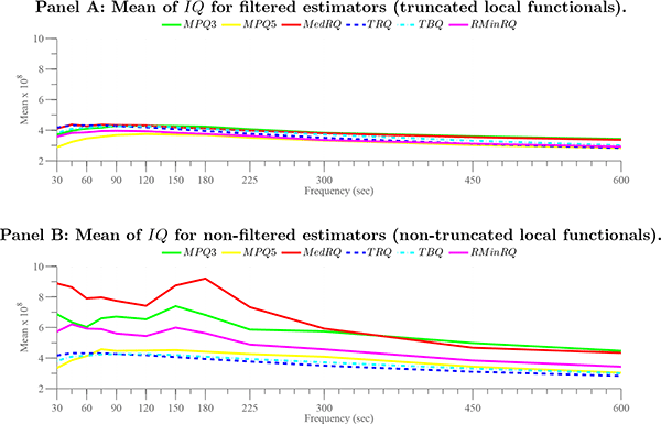
In Panel A, the estimation is performed as described in the paper and, in particular, all estimators, except TRQ and TBQ, are subject to the functional filtering procedure detailed in Section 4.3. In contrast, Panel B depicts the estimators without functional filtering. TRQ and TBQ are identical in the two panels, as they are based solely on truncation of individual returns. The average is across all stocks in the DJ30 index during January 2005-May 2007 and all estimates are pre-averaged and sub-sampled based on tick-time sampling.
Data for Figure 3, Panel A: Mean (x 10^8) of IQ for Filtered Estimators (Truncated Local Functionals)
| Frequency (sec) | MPQ3 | MPQ5 | MedRQ | TRQ | TBQ | RMinRQ |
|---|---|---|---|---|---|---|
| 30 | 3.720052514 | 2.882352867 | 4.112050783 | 4.169505815 | 3.818405666 | 3.577058332 |
| 45 | 3.96284425 | 3.233797842 | 4.365354983 | 4.328077841 | 4.097223671 | 3.817202615 |
| 60 | 4.102844248 | 3.463292385 | 4.263463079 | 4.308726968 | 4.158315036 | 3.858885348 |
| 75 | 4.167514311 | 3.571950206 | 4.361093916 | 4.312173156 | 4.248558974 | 3.94681871 |
| 90 | 4.286646907 | 3.676661753 | 4.331868069 | 4.269108127 | 4.264827533 | 3.960426747 |
| 120 | 4.296451455 | 3.74681628 | 4.315920155 | 4.190058557 | 4.266466997 | 3.930647661 |
| 150 | 4.271745768 | 3.705585243 | 4.189331996 | 4.065456989 | 4.195995383 | 3.833907777 |
| 180 | 4.234479083 | 3.691167127 | 4.119015655 | 3.942195463 | 4.092137306 | 3.750333772 |
| 225 | 4.063206141 | 3.506383059 | 3.967354564 | 3.77018488 | 3.934918866 | 3.626068863 |
| 300 | 3.82431234 | 3.322212776 | 3.792300309 | 3.504637654 | 3.715902125 | 3.351887742 |
| 450 | 3.597318717 | 3.02007369 | 3.547721962 | 3.106425695 | 3.31046994 | 3.118577729 |
| 600 | 3.429539062 | 2.833001672 | 3.368716961 | 2.836167193 | 3.002191115 | 2.917494906 |
Data for Figure 3, Panel B: Mean (x 10^8) of IQ for Non-Filtered Estimators (Non-Truncated Local Functionals)
| Frequency (sec) | MPQ3 | MPQ5 | MedRQ | TRQ | TBQ | RMinRQ |
|---|---|---|---|---|---|---|
| 30 | 6.87416483 | 3.348265637 | 8.884153873 | 4.169505815 | 3.818405666 | 5.727073845 |
| 45 | 6.349350447 | 3.85440939 | 8.63416259 | 4.328077841 | 4.097223671 | 6.204619289 |
| 60 | 6.03193449 | 4.1343941 | 7.899762717 | 4.308726968 | 4.158315036 | 5.923854596 |
| 75 | 6.593049391 | 4.572805461 | 7.964916605 | 4.312173156 | 4.248558974 | 5.891482615 |
| 90 | 6.70745045 | 4.467455878 | 7.749278786 | 4.269108127 | 4.264827533 | 5.609135727 |
| 120 | 6.534065317 | 4.487924556 | 7.419890263 | 4.190058557 | 4.266466997 | 5.441359872 |
| 150 | 7.393709164 | 4.523397832 | 8.74598091 | 4.065456989 | 4.195995383 | 5.98917296 |
| 180 | 6.818907836 | 4.41435621 | 9.198128198 | 3.942195463 | 4.092137306 | 5.627193569 |
| 225 | 5.85539223 | 4.261182136 | 7.3295521 | 3.77018488 | 3.934918866 | 4.884044066 |
| 300 | 5.743823156 | 4.088405367 | 5.923765616 | 3.504637654 | 3.715902125 | 4.573054409 |
| 450 | 4.983318115 | 3.436828686 | 4.677684464 | 3.106425695 | 3.31046994 | 3.841105603 |
| 600 | 4.47526915 | 3.041055095 | 4.339880334 | 2.836167193 | 3.002191115 | 3.437396771 |
Panel A of Figure 3 depicts signature plots for a group of IQ estimators, obtained by averaging the daily IQ estimates across the entire sample period and all of the thirty stocks. By construction, the figure speaks to mean and bias effects rather than efficiency. It shows that the estimators generally are quite similar although it also reveals some significant variation. First, at the highest frequencies a few estimators, especially MPQ5, appear severely downward biased. Hence, the noise-reduction associated with pre-averaging, sub-sampling and filtering has been successful in stemming the upward bias of the raw estimators. The remaining effects are consistent with the impact of irregular or sparse sampling of the returns at the highest frequencies, see Table 3, Panel H. The other striking feature is the slow decline in the plots as we move towards lower frequencies. The most likely explanation is the impact of time-varying volatility within the sampling interval, as indicated by the results in Table 3, Panels D and E. We pursue this issue in detail in the following section. Nonetheless, it is noteworthy that the signature plots are quite flat and largely coincide for the various estimators in the range of 90-150 seconds.
By contrast, Panel B of Figure 3 offers widely diverging results. Here, none of the estimators are subject to functional filtering, so only TRQ and TBQ provide uniform truncation of stark outliers. The consequence is apparent. Apart from the extreme dampening achieved by MPQ5, the remaining estimators are wildly upward biased at the higher frequencies. This speaks to the lack of robustness of IQ estimators that do not exploit direct truncation of individual returns. The problem of excessive variability, or noise, in IQ estimates has been noted sporadically in the empirical literature and it has motivated some authors to rely on low, and relatively inefficient but less error prone, frequencies for IQ estimation, e.g., BNS (2004a) and Bandi and Russell (2008). Similarly, Jiang and Oomen (2008) uses the squared IV as a simple approximation to IQ, thereby accepting a significant bias in exchange for variance reduction of the IQ estimator.
Thus, it is very encouraging that the functional filtering
regularizes the IQ estimators. The nominal size of our filter is
![]() , so only gross violations of the
Gaussian null is flagged. However, obviously, the null hypothesis
is not satisfied for actual high-frequency data, so the truncation
frequency is substantially larger in practice. For our equity data,
the fraction of observations filtered ranges from
, so only gross violations of the
Gaussian null is flagged. However, obviously, the null hypothesis
is not satisfied for actual high-frequency data, so the truncation
frequency is substantially larger in practice. For our equity data,
the fraction of observations filtered ranges from ![]() to
to ![]() for the 60-180 second range,
depending on the frequency and sample period. Overall, more than
70% of the stock days are untouched by our functional truncation.
In contrast, TBQ truncates at least one observation on 99.9% of the
days.26 Overall, the evidence is compatible
with our objective, namely that the functional filtering should
control major data irregularities while avoiding excessively
intrusive, and potentially distorting, truncation of the underlying
returns.
for the 60-180 second range,
depending on the frequency and sample period. Overall, more than
70% of the stock days are untouched by our functional truncation.
In contrast, TBQ truncates at least one observation on 99.9% of the
days.26 Overall, the evidence is compatible
with our objective, namely that the functional filtering should
control major data irregularities while avoiding excessively
intrusive, and potentially distorting, truncation of the underlying
returns.
6.2 The Intraday Volatility Pattern
One benefit of tick-time sampling of transactions data is that
it tends to mitigate the intra-day U-shape pattern in volatility.
Figure 4 demonstrates
that the tick-time sampling succeeds in straightening the
volatility pattern across the main part of the trading day, but
there is little impact on the elevated level of volatility in the
first 60-90 minutes of trading. Our Monte Carlo experiments found
such intraday volatility variation to be a potent source of
systematic biases in power variation estimates, with the ratio
statistic
![]() being less sensitive to such
distortions than the raw
being less sensitive to such
distortions than the raw ![]() and
and ![]() measures.
measures.
Figure 4: Diurnal volatility pattern for intraday trade data across the DJ30 stocks between January 1, 2005 and May 31, 2007.
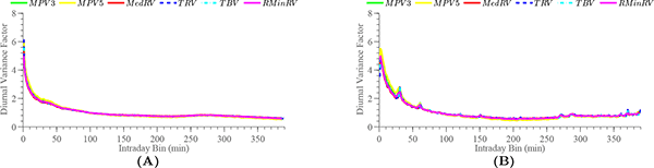
We plot the diurnal U-shape variance factors across stock-days based on local estimates
of
![]() in one minute buckets using tick
time (Panel A) or calendar time (Panel B) sampling. On each
stock-day, the factor in each one-minute bucket is computed by
normalizing by the average of the 390 variance estimates on that
day. The average variance factor is then computed by averaging
across all stock-days
in one minute buckets using tick
time (Panel A) or calendar time (Panel B) sampling. On each
stock-day, the factor in each one-minute bucket is computed by
normalizing by the average of the 390 variance estimates on that
day. The average variance factor is then computed by averaging
across all stock-days
Data for Figure 4, Panel A: Tick Time
| Intraday Bin (min) | MPV3 | MPV5 | MedRV | TRV | TBV | RMinRV |
|---|---|---|---|---|---|---|
| 1 | 6.064729982 | 6.022776011 | 5.341480764 | 6.164035434 | 5.777039144 | 5.004557031 |
| 2 | 4.613565484 | 4.882487692 | 4.169216556 | 4.454525454 | 4.403919085 | 4.142636973 |
| 3 | 4.084005134 | 4.337520533 | 3.673024203 | 3.890645523 | 3.891508601 | 3.714971954 |
| 4 | 3.780395522 | 3.937862803 | 3.403077789 | 3.517630798 | 3.570706647 | 3.426637816 |
| 5 | 3.506969572 | 3.677154387 | 3.221589471 | 3.364749558 | 3.374114756 | 3.233007102 |
| 6 | 3.267677058 | 3.499849224 | 3.012623121 | 3.163501366 | 3.173633628 | 3.065716301 |
| 7 | 3.093526251 | 3.324252024 | 2.828995683 | 2.993073099 | 2.963303811 | 2.89460483 |
| 8 | 2.959586019 | 3.235256365 | 2.7008724 | 2.798166335 | 2.840572381 | 2.777552384 |
| 9 | 2.843499457 | 3.043338114 | 2.616089934 | 2.701745173 | 2.745091074 | 2.674407739 |
| 10 | 2.753303917 | 2.921953112 | 2.541200946 | 2.642641651 | 2.63482782 | 2.593835087 |
| 11 | 2.607607721 | 2.830135698 | 2.40635473 | 2.526060076 | 2.550188722 | 2.495426477 |
| 12 | 2.527600851 | 2.692385034 | 2.362544699 | 2.448782731 | 2.446077956 | 2.412963322 |
| 13 | 2.44955126 | 2.572271387 | 2.27571698 | 2.333683131 | 2.358744897 | 2.326788387 |
| 14 | 2.384465484 | 2.523862332 | 2.214671271 | 2.314846403 | 2.336624934 | 2.260742323 |
| 15 | 2.284930017 | 2.41514381 | 2.163225949 | 2.269376317 | 2.252272265 | 2.197086703 |
| 16 | 2.219770939 | 2.361207251 | 2.062121631 | 2.153187051 | 2.143612188 | 2.137509463 |
| 17 | 2.154926618 | 2.323151138 | 2.045166434 | 2.134803291 | 2.150363973 | 2.12183224 |
| 18 | 2.12863631 | 2.281723383 | 1.979768603 | 2.098052291 | 2.056446669 | 2.075473317 |
| 19 | 2.08747205 | 2.210894078 | 1.953128198 | 1.987996162 | 2.012154711 | 2.033085551 |
| 20 | 2.077482269 | 2.190707709 | 1.96420105 | 1.994568794 | 2.028905116 | 2.009589393 |
| 21 | 2.041917845 | 2.184298198 | 1.924936855 | 1.988238035 | 2.004059556 | 1.979040903 |
| 22 | 2.018129197 | 2.141443598 | 1.910358598 | 1.965989605 | 1.967640645 | 1.955905014 |
| 23 | 1.993637509 | 2.07286322 | 1.880109851 | 1.901085625 | 1.941615837 | 1.920921853 |
| 24 | 1.948927115 | 2.028504283 | 1.828125057 | 1.864218195 | 1.90552374 | 1.884011271 |
| 25 | 1.904632673 | 2.016084587 | 1.807464668 | 1.874103006 | 1.896089194 | 1.852760088 |
| 26 | 1.849826117 | 1.968689969 | 1.761693733 | 1.831899175 | 1.828594129 | 1.834099072 |
| 27 | 1.829757518 | 1.958663154 | 1.736175711 | 1.780875062 | 1.78428099 | 1.800323376 |
| 28 | 1.82491881 | 1.930477232 | 1.724054015 | 1.769055121 | 1.776376324 | 1.78789884 |
| 29 | 1.827960611 | 1.954213682 | 1.716579262 | 1.760321616 | 1.763630811 | 1.777254617 |
| 30 | 1.8209282 | 1.968023005 | 1.709991848 | 1.721954478 | 1.76720133 | 1.779292681 |
| 31 | 1.804548083 | 1.962643952 | 1.714283934 | 1.727049299 | 1.761461176 | 1.778709346 |
| 32 | 1.801821742 | 1.915146493 | 1.702068939 | 1.753121313 | 1.748199099 | 1.765887984 |
| 33 | 1.795758994 | 1.876877507 | 1.702644778 | 1.662108498 | 1.727391864 | 1.757239536 |
| 34 | 1.79778912 | 1.869808156 | 1.709012691 | 1.729752976 | 1.750542213 | 1.741131745 |
| 35 | 1.752540222 | 1.855105318 | 1.70199856 | 1.716478522 | 1.736422154 | 1.726154209 |
| 36 | 1.726994938 | 1.840855521 | 1.643513403 | 1.69513222 | 1.690101947 | 1.714808957 |
| 37 | 1.694095711 | 1.856223734 | 1.631958524 | 1.681018864 | 1.672103811 | 1.710465175 |
| 38 | 1.721163978 | 1.836336679 | 1.629358835 | 1.635864252 | 1.636273486 | 1.688399664 |
| 39 | 1.72436076 | 1.788772264 | 1.631005903 | 1.635711574 | 1.676229061 | 1.683861655 |
| 40 | 1.705467333 | 1.809832904 | 1.623944847 | 1.66134682 | 1.680092318 | 1.679422869 |
| 41 | 1.660650218 | 1.791071363 | 1.578582792 | 1.644143242 | 1.638521649 | 1.653240657 |
| 42 | 1.683891311 | 1.769933551 | 1.597288334 | 1.589464952 | 1.597020722 | 1.626355896 |
| 43 | 1.680157348 | 1.7531881 | 1.594193687 | 1.579436933 | 1.640393218 | 1.606804628 |
| 44 | 1.654379468 | 1.723502436 | 1.561082818 | 1.619203232 | 1.628674094 | 1.587814124 |
| 45 | 1.593169138 | 1.664343538 | 1.533317966 | 1.549926713 | 1.564845776 | 1.558810123 |
| 46 | 1.565620551 | 1.634144283 | 1.516620091 | 1.523269948 | 1.538248256 | 1.537039869 |
| 47 | 1.524130087 | 1.604629903 | 1.488526042 | 1.499681391 | 1.502518185 | 1.516667073 |
| 48 | 1.522978048 | 1.599818722 | 1.480837745 | 1.486209955 | 1.495305177 | 1.497418333 |
| 49 | 1.513444478 | 1.572962598 | 1.442312163 | 1.467533618 | 1.486847493 | 1.468895612 |
| 50 | 1.483929856 | 1.551094663 | 1.418349876 | 1.454030072 | 1.458162533 | 1.456255108 |
| 51 | 1.474694267 | 1.537144598 | 1.397262004 | 1.419461809 | 1.447853838 | 1.442377522 |
| 52 | 1.449493739 | 1.496033654 | 1.377755252 | 1.402583829 | 1.409665643 | 1.427677699 |
| 53 | 1.425656454 | 1.481856932 | 1.389670032 | 1.378111143 | 1.411060539 | 1.399687103 |
| 54 | 1.420637605 | 1.465760587 | 1.365262103 | 1.382436403 | 1.394402854 | 1.386084074 |
| 55 | 1.39778158 | 1.438308217 | 1.351397355 | 1.376732392 | 1.385432775 | 1.367253583 |
| 56 | 1.375205613 | 1.400733665 | 1.315731151 | 1.355752551 | 1.355041385 | 1.33726062 |
| 57 | 1.330809327 | 1.374923611 | 1.302294972 | 1.312109051 | 1.330563902 | 1.316620474 |
| 58 | 1.321031456 | 1.377600697 | 1.276626229 | 1.302223255 | 1.307406951 | 1.313068879 |
| 59 | 1.299486101 | 1.351832209 | 1.264951513 | 1.300893959 | 1.286863667 | 1.308990925 |
| 60 | 1.307347206 | 1.343865335 | 1.268215957 | 1.260610089 | 1.277584017 | 1.298476334 |
| 61 | 1.318354422 | 1.361837511 | 1.269006212 | 1.27571242 | 1.299444804 | 1.299428313 |
| 62 | 1.288785753 | 1.355890605 | 1.270342929 | 1.274801086 | 1.286946821 | 1.288077696 |
| 63 | 1.293812028 | 1.347095813 | 1.271605672 | 1.252751242 | 1.269503556 | 1.284965186 |
| 64 | 1.298657247 | 1.349930462 | 1.260809332 | 1.261070125 | 1.276610497 | 1.292905736 |
| 65 | 1.293666032 | 1.331554438 | 1.25821166 | 1.261697157 | 1.27920466 | 1.277354777 |
| 66 | 1.290083641 | 1.301687497 | 1.246686877 | 1.245738999 | 1.259321623 | 1.27038105 |
| 67 | 1.25468691 | 1.294865077 | 1.244572873 | 1.247926202 | 1.25945725 | 1.256375147 |
| 68 | 1.26577821 | 1.305356313 | 1.232668255 | 1.236556587 | 1.236907937 | 1.259125339 |
| 69 | 1.251988057 | 1.276933223 | 1.224568964 | 1.208649929 | 1.237079825 | 1.237755853 |
| 70 | 1.259512277 | 1.280212295 | 1.226165306 | 1.218090515 | 1.235300782 | 1.226836822 |
| 71 | 1.229897737 | 1.247469223 | 1.210250172 | 1.223270051 | 1.246310079 | 1.222111696 |
| 72 | 1.221010848 | 1.241222012 | 1.190503769 | 1.227629561 | 1.213757218 | 1.202002821 |
| 73 | 1.185878762 | 1.217340485 | 1.161583531 | 1.160935262 | 1.17173275 | 1.202463482 |
| 74 | 1.204479608 | 1.213876044 | 1.188381427 | 1.178127296 | 1.190187185 | 1.209053522 |
| 75 | 1.198479256 | 1.205152157 | 1.194933179 | 1.172162943 | 1.199233582 | 1.205409648 |
| 76 | 1.192342893 | 1.189468461 | 1.194437691 | 1.186185689 | 1.189668885 | 1.19153043 |
| 77 | 1.185546332 | 1.19194341 | 1.160545584 | 1.177928366 | 1.189120285 | 1.187227057 |
| 78 | 1.171534703 | 1.19143832 | 1.168068298 | 1.169158836 | 1.171684011 | 1.179937998 |
| 79 | 1.171392307 | 1.187703893 | 1.144432968 | 1.140946143 | 1.154657707 | 1.159661812 |
| 80 | 1.157895167 | 1.175767035 | 1.125309332 | 1.125993087 | 1.140843741 | 1.147873068 |
| 81 | 1.155529186 | 1.161841365 | 1.150080206 | 1.158953531 | 1.148227195 | 1.144739957 |
| 82 | 1.142085436 | 1.153346688 | 1.129121639 | 1.121672526 | 1.130633208 | 1.138589997 |
| 83 | 1.143299601 | 1.168033265 | 1.129155109 | 1.135443789 | 1.140109003 | 1.129968589 |
| 84 | 1.118995223 | 1.144210787 | 1.0997482 | 1.108420975 | 1.11408785 | 1.114175711 |
| 85 | 1.123980789 | 1.149215482 | 1.102230807 | 1.109245344 | 1.120863574 | 1.106935542 |
| 86 | 1.112133561 | 1.134469474 | 1.099104823 | 1.083770288 | 1.097256208 | 1.107082411 |
| 87 | 1.119038941 | 1.137165223 | 1.100659058 | 1.086746639 | 1.116358466 | 1.09897768 |
| 88 | 1.09892889 | 1.117556787 | 1.086778373 | 1.084272471 | 1.093938899 | 1.093015162 |
| 89 | 1.099424907 | 1.085823016 | 1.078557306 | 1.062903217 | 1.080136096 | 1.087617609 |
| 90 | 1.080745505 | 1.071731821 | 1.073932646 | 1.068679712 | 1.084140203 | 1.072073304 |
| 91 | 1.054665259 | 1.075511854 | 1.059165357 | 1.06859905 | 1.069260244 | 1.059772617 |
| 92 | 1.045655426 | 1.048687165 | 1.049740324 | 1.05256547 | 1.047980326 | 1.053186407 |
| 93 | 1.039679399 | 1.039578387 | 1.039864115 | 1.019436545 | 1.035901017 | 1.03844283 |
| 94 | 1.04827344 | 1.041724905 | 1.048854607 | 1.031448906 | 1.049629749 | 1.039747391 |
| 95 | 1.026012176 | 1.006883455 | 1.031169757 | 1.013641328 | 1.03425028 | 1.020822009 |
| 96 | 1.011951973 | 1.0027134 | 1.020311474 | 1.023801037 | 1.019975637 | 1.021228394 |
| 97 | 0.9967061 | 0.981609944 | 1.009224404 | 1.003939262 | 1.008563811 | 1.005281682 |
| 98 | 0.993736328 | 0.985098088 | 1.000389978 | 1.003754132 | 1.006866834 | 0.9958858 |
| 99 | 0.971389736 | 0.962382956 | 0.978318433 | 0.989256488 | 0.982428382 | 0.988425397 |
| 100 | 0.968371996 | 0.949000372 | 0.974232537 | 0.968263118 | 0.974366209 | 0.976644143 |
| 101 | 0.953848606 | 0.946874781 | 0.968067979 | 0.972655564 | 0.969487847 | 0.978709256 |
| 102 | 0.957184032 | 0.945686181 | 0.97278091 | 0.959370092 | 0.960072564 | 0.970273096 |
| 103 | 0.956515717 | 0.947521893 | 0.968337996 | 0.961392298 | 0.960478987 | 0.967900011 |
| 104 | 0.951682285 | 0.944712877 | 0.96050819 | 0.957015126 | 0.966223412 | 0.957089644 |
| 105 | 0.943032276 | 0.939303924 | 0.952551213 | 0.965105613 | 0.951822488 | 0.957762808 |
| 106 | 0.936691126 | 0.925204159 | 0.94534084 | 0.937622548 | 0.933321244 | 0.952604519 |
| 107 | 0.950569044 | 0.942597283 | 0.955318297 | 0.942161629 | 0.948424628 | 0.95702096 |
| 108 | 0.947249606 | 0.941338958 | 0.946728019 | 0.939271888 | 0.949692738 | 0.949404478 |
| 109 | 0.940845251 | 0.923357094 | 0.940369439 | 0.937103432 | 0.938489657 | 0.947005163 |
| 110 | 0.931787438 | 0.912509282 | 0.947118484 | 0.938400888 | 0.946730917 | 0.937194578 |
| 111 | 0.919546132 | 0.907975835 | 0.932147092 | 0.938762625 | 0.930217837 | 0.933039272 |
| 112 | 0.915751057 | 0.907403985 | 0.923828675 | 0.922596305 | 0.920179574 | 0.927793983 |
| 113 | 0.900918837 | 0.908106074 | 0.924045875 | 0.916468631 | 0.920294033 | 0.929196967 |
| 114 | 0.908368862 | 0.905297304 | 0.92863022 | 0.920312278 | 0.915984867 | 0.922235378 |
| 115 | 0.911626769 | 0.888801568 | 0.927236323 | 0.913708117 | 0.912590259 | 0.91293104 |
| 116 | 0.905056274 | 0.894860591 | 0.92736248 | 0.918776142 | 0.914643811 | 0.917057282 |
| 117 | 0.892888437 | 0.891278446 | 0.919487338 | 0.916132405 | 0.908235461 | 0.907461917 |
| 118 | 0.896021885 | 0.875275499 | 0.911604378 | 0.889454058 | 0.891751049 | 0.895213474 |
| 119 | 0.884495764 | 0.878596989 | 0.901594507 | 0.892556748 | 0.904905186 | 0.899203312 |
| 120 | 0.88152932 | 0.859240337 | 0.906352479 | 0.91724525 | 0.888595627 | 0.902006957 |
| 121 | 0.893545457 | 0.870482303 | 0.902529343 | 0.875673143 | 0.882901964 | 0.898888702 |
| 122 | 0.876513005 | 0.875935268 | 0.893604843 | 0.89196468 | 0.899328114 | 0.891797054 |
| 123 | 0.890489284 | 0.883262093 | 0.897340468 | 0.897219576 | 0.882568507 | 0.886834878 |
| 124 | 0.870069857 | 0.865019374 | 0.875506965 | 0.872642427 | 0.88685755 | 0.883431908 |
| 125 | 0.878516602 | 0.849982686 | 0.886518357 | 0.886240983 | 0.875397979 | 0.878441833 |
| 126 | 0.859183433 | 0.829321726 | 0.887258383 | 0.869301727 | 0.868635947 | 0.868393284 |
| 127 | 0.861100811 | 0.841741021 | 0.886180893 | 0.875101675 | 0.877682463 | 0.871753446 |
| 128 | 0.852099254 | 0.84554405 | 0.860411265 | 0.875520073 | 0.867128015 | 0.861473148 |
| 129 | 0.843807057 | 0.825773208 | 0.863475772 | 0.861142461 | 0.847249051 | 0.856944107 |
| 130 | 0.847052819 | 0.811539221 | 0.860772967 | 0.844544964 | 0.85043947 | 0.853047368 |
| 131 | 0.83600604 | 0.812427864 | 0.86189307 | 0.869320202 | 0.857680568 | 0.853149861 |
| 132 | 0.826709184 | 0.808181836 | 0.859146085 | 0.849315342 | 0.839745665 | 0.852726988 |
| 133 | 0.841257808 | 0.817022673 | 0.85375294 | 0.844851696 | 0.847637075 | 0.854355832 |
| 134 | 0.832855286 | 0.817897165 | 0.863423161 | 0.855863054 | 0.849515503 | 0.850458881 |
| 135 | 0.836445373 | 0.82715027 | 0.859568879 | 0.85242015 | 0.845832346 | 0.854978339 |
| 136 | 0.835598529 | 0.810082212 | 0.860782936 | 0.836543521 | 0.837792724 | 0.854570271 |
| 137 | 0.845045019 | 0.798277578 | 0.862702055 | 0.844706495 | 0.845188038 | 0.845369992 |
| 138 | 0.826888779 | 0.785944284 | 0.855120991 | 0.845098721 | 0.851516266 | 0.833210663 |
| 139 | 0.815683465 | 0.80061502 | 0.841967645 | 0.854975646 | 0.844419422 | 0.835346239 |
| 140 | 0.799920634 | 0.793972006 | 0.822677097 | 0.826878209 | 0.812962358 | 0.833865326 |
| 141 | 0.815003329 | 0.797957185 | 0.829796518 | 0.812139555 | 0.81309233 | 0.825632701 |
| 142 | 0.825488397 | 0.783410793 | 0.843999378 | 0.820415874 | 0.831382135 | 0.829929208 |
| 143 | 0.819858468 | 0.795240667 | 0.838245629 | 0.834383062 | 0.843045808 | 0.834388201 |
| 144 | 0.805588925 | 0.768551516 | 0.831755999 | 0.846772487 | 0.830475868 | 0.831056887 |
| 145 | 0.809517499 | 0.772069863 | 0.830961121 | 0.808239732 | 0.804789775 | 0.827452565 |
| 146 | 0.801261928 | 0.793784593 | 0.838821987 | 0.80750168 | 0.822401529 | 0.836256783 |
| 147 | 0.82495157 | 0.805368721 | 0.847815077 | 0.837689051 | 0.828277019 | 0.838136195 |
| 148 | 0.824620796 | 0.788932237 | 0.84464601 | 0.814242684 | 0.826865528 | 0.827387703 |
| 149 | 0.824146438 | 0.795928697 | 0.857700897 | 0.834724103 | 0.840506119 | 0.831899375 |
| 150 | 0.799897279 | 0.775963122 | 0.829121055 | 0.837067286 | 0.835825794 | 0.824302519 |
| 151 | 0.802750819 | 0.773381792 | 0.822124473 | 0.824288129 | 0.805052776 | 0.817697271 |
| 152 | 0.80583139 | 0.786465382 | 0.825807395 | 0.809805757 | 0.815594016 | 0.815136684 |
| 153 | 0.807289829 | 0.771256268 | 0.834198133 | 0.823422704 | 0.817919441 | 0.814601707 |
| 154 | 0.810736041 | 0.772401631 | 0.830012435 | 0.819232534 | 0.818750099 | 0.818803572 |
| 155 | 0.791516777 | 0.767774302 | 0.822862171 | 0.81349675 | 0.820256107 | 0.815635264 |
| 156 | 0.801170638 | 0.769035635 | 0.823248387 | 0.801841662 | 0.804438129 | 0.816335912 |
| 157 | 0.810644072 | 0.783220422 | 0.824940183 | 0.798646475 | 0.811504185 | 0.813556428 |
| 158 | 0.801506517 | 0.771156809 | 0.818751667 | 0.802753957 | 0.81766244 | 0.810442138 |
| 159 | 0.796546252 | 0.766177487 | 0.821081351 | 0.809971122 | 0.806362468 | 0.802724873 |
| 160 | 0.79633251 | 0.786544112 | 0.823263515 | 0.810192519 | 0.810639282 | 0.807735225 |
| 161 | 0.790320203 | 0.78812903 | 0.818563732 | 0.814772075 | 0.807773475 | 0.81899645 |
| 162 | 0.795030761 | 0.771412636 | 0.824419999 | 0.80263092 | 0.793480396 | 0.809171469 |
| 163 | 0.80942368 | 0.781770459 | 0.831656302 | 0.801387371 | 0.811754311 | 0.816424389 |
| 164 | 0.798488408 | 0.777559967 | 0.823876318 | 0.810782265 | 0.822671438 | 0.81634541 |
| 165 | 0.799620945 | 0.7676444 | 0.819209495 | 0.820168813 | 0.807114228 | 0.810436639 |
| 166 | 0.792101932 | 0.748705153 | 0.819270321 | 0.785906945 | 0.794918029 | 0.800923558 |
| 167 | 0.796488195 | 0.771857297 | 0.823007314 | 0.822127762 | 0.81804312 | 0.80522581 |
| 168 | 0.774522098 | 0.748778909 | 0.807115971 | 0.796378409 | 0.792972881 | 0.799616081 |
| 169 | 0.782631228 | 0.752501124 | 0.809227844 | 0.8001179 | 0.789468962 | 0.805222349 |
| 170 | 0.783406686 | 0.755363339 | 0.824057884 | 0.788813022 | 0.802392734 | 0.810455244 |
| 171 | 0.790764199 | 0.755879707 | 0.818496701 | 0.80761689 | 0.804345907 | 0.807547645 |
| 172 | 0.789714373 | 0.750866432 | 0.820287783 | 0.788667001 | 0.798303065 | 0.800719339 |
| 173 | 0.776878935 | 0.741981159 | 0.810681353 | 0.798663042 | 0.801644364 | 0.794831858 |
| 174 | 0.768422167 | 0.735961756 | 0.806382769 | 0.809576749 | 0.791878825 | 0.793535325 |
| 175 | 0.763099093 | 0.725927283 | 0.791449046 | 0.778875676 | 0.768222822 | 0.795691515 |
| 176 | 0.770208394 | 0.745941262 | 0.806199915 | 0.790335914 | 0.789589798 | 0.791025915 |
| 177 | 0.765504707 | 0.755518384 | 0.809102865 | 0.78618778 | 0.78433895 | 0.785809907 |
| 178 | 0.763959987 | 0.761806453 | 0.797235701 | 0.78048978 | 0.783468508 | 0.788570012 |
| 179 | 0.765175309 | 0.746465029 | 0.797024361 | 0.795250333 | 0.774233069 | 0.787324527 |
| 180 | 0.771033939 | 0.735430035 | 0.794168874 | 0.765381411 | 0.778453255 | 0.786789645 |
| 181 | 0.770998996 | 0.73857868 | 0.803203832 | 0.790693926 | 0.790311687 | 0.785483116 |
| 182 | 0.763796547 | 0.742068462 | 0.796044354 | 0.787764961 | 0.784795036 | 0.784174736 |
| 183 | 0.769139576 | 0.752261063 | 0.79444705 | 0.796242265 | 0.784058517 | 0.779292189 |
| 184 | 0.761126405 | 0.721558996 | 0.783198679 | 0.761419684 | 0.758739334 | 0.771811777 |
| 185 | 0.756472882 | 0.7378471 | 0.787375637 | 0.763550895 | 0.775797718 | 0.771953847 |
| 186 | 0.75815827 | 0.733278601 | 0.793492436 | 0.779570791 | 0.778638459 | 0.779666934 |
| 187 | 0.757566326 | 0.72727677 | 0.786527206 | 0.778938372 | 0.772146932 | 0.779235158 |
| 188 | 0.748070667 | 0.712381159 | 0.786536514 | 0.780806113 | 0.764763221 | 0.77383896 |
| 189 | 0.753077944 | 0.69306916 | 0.787111383 | 0.76174315 | 0.76154787 | 0.764478624 |
| 190 | 0.758121132 | 0.697179223 | 0.789678025 | 0.769656243 | 0.779539907 | 0.760095831 |
| 191 | 0.727964876 | 0.703754535 | 0.770057482 | 0.773389905 | 0.763224126 | 0.757549789 |
| 192 | 0.731935364 | 0.716864826 | 0.770582762 | 0.765775764 | 0.747632228 | 0.756720545 |
| 193 | 0.740165119 | 0.700248257 | 0.771500451 | 0.74494325 | 0.747170305 | 0.751370502 |
| 194 | 0.747018152 | 0.700157378 | 0.769920822 | 0.752237906 | 0.761584709 | 0.749525999 |
| 195 | 0.730186823 | 0.699058925 | 0.76822291 | 0.767636665 | 0.753983136 | 0.748543379 |
| 196 | 0.726920289 | 0.691692039 | 0.770982136 | 0.753581786 | 0.753761703 | 0.754777637 |
| 197 | 0.732109332 | 0.689367452 | 0.764687408 | 0.749727461 | 0.742542324 | 0.747376838 |
| 198 | 0.7396009 | 0.70607879 | 0.770624807 | 0.739174995 | 0.752964177 | 0.752111784 |
| 199 | 0.722494414 | 0.692891141 | 0.769103231 | 0.745350664 | 0.749128981 | 0.75458529 |
| 200 | 0.736743783 | 0.704207834 | 0.760069531 | 0.754852562 | 0.739002533 | 0.751883888 |
| 201 | 0.72560778 | 0.684609961 | 0.758871559 | 0.741075495 | 0.750597421 | 0.747181355 |
| 202 | 0.732635676 | 0.684512764 | 0.755819751 | 0.756917091 | 0.742906872 | 0.746651362 |
| 203 | 0.725783898 | 0.692984379 | 0.759344726 | 0.747251286 | 0.744839233 | 0.73941781 |
| 204 | 0.723565054 | 0.698320317 | 0.762968878 | 0.748161258 | 0.742867458 | 0.741150631 |
| 205 | 0.715656539 | 0.689702773 | 0.751205281 | 0.733179949 | 0.733732041 | 0.736818 |
| 206 | 0.72530679 | 0.672144964 | 0.75523153 | 0.745463834 | 0.736043368 | 0.729750818 |
| 207 | 0.714763353 | 0.673552882 | 0.756679847 | 0.738543964 | 0.742267425 | 0.727991879 |
| 208 | 0.710136698 | 0.688702643 | 0.752598703 | 0.739347926 | 0.736682025 | 0.732834782 |
| 209 | 0.707496749 | 0.684958312 | 0.747603398 | 0.742349361 | 0.724954416 | 0.733734832 |
| 210 | 0.71021615 | 0.681324702 | 0.747461154 | 0.730027269 | 0.715212166 | 0.735428949 |
| 211 | 0.721557346 | 0.679849841 | 0.754194033 | 0.727636116 | 0.733036984 | 0.73929539 |
| 212 | 0.719396971 | 0.677771059 | 0.75600904 | 0.743048897 | 0.738328092 | 0.739517569 |
| 213 | 0.71552984 | 0.673250702 | 0.757872044 | 0.747078074 | 0.732347489 | 0.73946054 |
| 214 | 0.712606062 | 0.675214693 | 0.753597143 | 0.74144773 | 0.736000154 | 0.733241278 |
| 215 | 0.705757861 | 0.672774779 | 0.757921408 | 0.74834308 | 0.732629724 | 0.73163258 |
| 216 | 0.711227695 | 0.681361498 | 0.745463116 | 0.728643619 | 0.72433668 | 0.732808981 |
| 217 | 0.71422595 | 0.683571932 | 0.749042261 | 0.731959289 | 0.730090532 | 0.73032651 |
| 218 | 0.714554462 | 0.678938189 | 0.75371688 | 0.725708665 | 0.728309363 | 0.732267782 |
| 219 | 0.722238669 | 0.668623725 | 0.760913922 | 0.742467353 | 0.741341369 | 0.72877607 |
| 220 | 0.711475538 | 0.664580987 | 0.742708379 | 0.74518694 | 0.735487894 | 0.732044404 |
| 221 | 0.704018366 | 0.661464323 | 0.745329668 | 0.730516123 | 0.726333651 | 0.727558795 |
| 222 | 0.703983061 | 0.668488077 | 0.74714143 | 0.741732871 | 0.723568304 | 0.728486886 |
| 223 | 0.704815315 | 0.678116015 | 0.747948811 | 0.706607449 | 0.71671718 | 0.727333085 |
| 224 | 0.711474116 | 0.692602938 | 0.755281134 | 0.74134977 | 0.738146918 | 0.734206756 |
| 225 | 0.729332401 | 0.69686167 | 0.755100824 | 0.736000902 | 0.735949443 | 0.736668969 |
| 226 | 0.72365209 | 0.68558394 | 0.753752513 | 0.740282437 | 0.741416543 | 0.736252272 |
| 227 | 0.722324029 | 0.680268364 | 0.749672789 | 0.73889908 | 0.738902535 | 0.737165538 |
| 228 | 0.708693248 | 0.672480064 | 0.753324901 | 0.739233344 | 0.732959765 | 0.741420174 |
| 229 | 0.711341994 | 0.67295485 | 0.751481086 | 0.740232371 | 0.732356962 | 0.73966533 |
| 230 | 0.713001139 | 0.681411138 | 0.757455997 | 0.734527042 | 0.732270839 | 0.739731108 |
| 231 | 0.717126885 | 0.686113311 | 0.755177122 | 0.732418851 | 0.730251358 | 0.741157651 |
| 232 | 0.726996798 | 0.694392242 | 0.755182066 | 0.741343369 | 0.741966788 | 0.74961419 |
| 233 | 0.726442625 | 0.691494129 | 0.764038723 | 0.740334104 | 0.740239725 | 0.750321262 |
| 234 | 0.733868339 | 0.701113962 | 0.765863077 | 0.74689107 | 0.746395483 | 0.753416194 |
| 235 | 0.725243512 | 0.693252887 | 0.764984625 | 0.745005908 | 0.74286371 | 0.750820821 |
| 236 | 0.733793373 | 0.696554958 | 0.776542216 | 0.752103051 | 0.746773773 | 0.756333778 |
| 237 | 0.731326801 | 0.697136578 | 0.76992454 | 0.756926734 | 0.748553778 | 0.756585036 |
| 238 | 0.73522597 | 0.70417305 | 0.776090814 | 0.759539148 | 0.747213093 | 0.754346293 |
| 239 | 0.72892768 | 0.699419599 | 0.772645498 | 0.748384549 | 0.748752133 | 0.753923998 |
| 240 | 0.730874103 | 0.698029852 | 0.762713892 | 0.758753543 | 0.749388759 | 0.747529423 |
| 241 | 0.732115141 | 0.707933596 | 0.768879711 | 0.75783636 | 0.747586108 | 0.751752562 |
| 242 | 0.737675213 | 0.718732496 | 0.767065803 | 0.748790104 | 0.750438027 | 0.759170832 |
| 243 | 0.748309472 | 0.723406253 | 0.771682379 | 0.757438307 | 0.753800611 | 0.766144863 |
| 244 | 0.752277014 | 0.737382944 | 0.783838935 | 0.765581881 | 0.76549259 | 0.764509581 |
| 245 | 0.761548243 | 0.749976176 | 0.779780011 | 0.766805002 | 0.767800682 | 0.770983613 |
| 246 | 0.758331607 | 0.734525368 | 0.778422008 | 0.765226835 | 0.765853297 | 0.779437975 |
| 247 | 0.7758565 | 0.753128532 | 0.797363746 | 0.776931127 | 0.77780327 | 0.783209634 |
| 248 | 0.772245641 | 0.758136531 | 0.801800518 | 0.781634738 | 0.787598832 | 0.786517336 |
| 249 | 0.77018602 | 0.740718735 | 0.791404385 | 0.78064799 | 0.778969291 | 0.781613572 |
| 250 | 0.778920674 | 0.744488087 | 0.791835895 | 0.778530471 | 0.778328544 | 0.781939615 |
| 251 | 0.768856676 | 0.74800365 | 0.794156065 | 0.779404466 | 0.788596242 | 0.782885554 |
| 252 | 0.769160916 | 0.757548917 | 0.794494325 | 0.779040368 | 0.776600752 | 0.787909771 |
| 253 | 0.781742694 | 0.770388824 | 0.794888 | 0.773877659 | 0.787697085 | 0.794147093 |
| 254 | 0.778390302 | 0.757114712 | 0.807580522 | 0.784963753 | 0.780582657 | 0.803786303 |
| 255 | 0.794003138 | 0.772869962 | 0.809106077 | 0.785764518 | 0.801840087 | 0.800424627 |
| 256 | 0.78800507 | 0.752950352 | 0.810067711 | 0.803811303 | 0.800124515 | 0.80619084 |
| 257 | 0.788871929 | 0.75589208 | 0.815359773 | 0.801245313 | 0.804298575 | 0.80296775 |
| 258 | 0.778327358 | 0.766121679 | 0.810928941 | 0.802381227 | 0.793653386 | 0.809616845 |
| 259 | 0.77613774 | 0.767702908 | 0.811986675 | 0.794092355 | 0.79145535 | 0.806077604 |
| 260 | 0.796891336 | 0.770939628 | 0.829229024 | 0.810114044 | 0.796743301 | 0.813092861 |
| 261 | 0.796664496 | 0.778155287 | 0.824496405 | 0.802153424 | 0.814096116 | 0.815027233 |
| 262 | 0.797537534 | 0.794524113 | 0.826368909 | 0.825327671 | 0.811664485 | 0.818563749 |
| 263 | 0.80448571 | 0.793319863 | 0.831739534 | 0.801805373 | 0.807060296 | 0.823500396 |
| 264 | 0.815389831 | 0.785021437 | 0.83143744 | 0.81763527 | 0.825516724 | 0.823060058 |
| 265 | 0.807100672 | 0.783392389 | 0.83486675 | 0.814872917 | 0.816904537 | 0.82303206 |
| 266 | 0.799381212 | 0.781586213 | 0.831639234 | 0.807269459 | 0.812854029 | 0.81709168 |
| 267 | 0.807840593 | 0.793407074 | 0.834747242 | 0.814982005 | 0.814606227 | 0.818597005 |
| 268 | 0.797534497 | 0.782319727 | 0.820570968 | 0.812340506 | 0.810555598 | 0.822429697 |
| 269 | 0.80651888 | 0.793971914 | 0.828241083 | 0.820020386 | 0.813025641 | 0.822157793 |
| 270 | 0.801242504 | 0.790225575 | 0.832571616 | 0.810624522 | 0.814870613 | 0.818814151 |
| 271 | 0.805268447 | 0.786469455 | 0.834779992 | 0.826125259 | 0.813434465 | 0.821924778 |
| 272 | 0.8044399 | 0.772822724 | 0.827440095 | 0.814722378 | 0.819021163 | 0.816374685 |
| 273 | 0.793560664 | 0.768924415 | 0.829096233 | 0.821354504 | 0.818960845 | 0.822306853 |
| 274 | 0.791469812 | 0.769872886 | 0.823518352 | 0.805747037 | 0.79474911 | 0.822432825 |
| 275 | 0.790971963 | 0.767357003 | 0.827681681 | 0.802145554 | 0.803436619 | 0.817247738 |
| 276 | 0.810184568 | 0.78557662 | 0.829909188 | 0.808248431 | 0.816206406 | 0.821888184 |
| 277 | 0.803828835 | 0.790908752 | 0.824182983 | 0.823453456 | 0.826625947 | 0.824336273 |
| 278 | 0.806535897 | 0.794499184 | 0.821806097 | 0.81745532 | 0.803051413 | 0.824904718 |
| 279 | 0.807057485 | 0.801363789 | 0.833002052 | 0.79886399 | 0.811644421 | 0.818277809 |
| 280 | 0.810065326 | 0.788497318 | 0.836925056 | 0.817719666 | 0.825151524 | 0.818176496 |
| 281 | 0.809096508 | 0.789770926 | 0.824751057 | 0.833592683 | 0.817560003 | 0.81646948 |
| 282 | 0.790306114 | 0.772886176 | 0.815164685 | 0.795659969 | 0.801616318 | 0.809036043 |
| 283 | 0.80031496 | 0.779340595 | 0.828759084 | 0.807680397 | 0.804660894 | 0.814804529 |
| 284 | 0.803457611 | 0.782926745 | 0.814682959 | 0.794423084 | 0.806683508 | 0.80335104 |
| 285 | 0.807374608 | 0.768519445 | 0.815257338 | 0.81416603 | 0.808662462 | 0.805116384 |
| 286 | 0.789859669 | 0.759489556 | 0.812047221 | 0.79281351 | 0.796712414 | 0.800141057 |
| 287 | 0.779450186 | 0.751598245 | 0.813516501 | 0.794882726 | 0.801857289 | 0.802910157 |
| 288 | 0.781148898 | 0.747712062 | 0.810888313 | 0.804078399 | 0.793851359 | 0.7988179 |
| 289 | 0.771726718 | 0.739393763 | 0.804640696 | 0.781748199 | 0.791482834 | 0.799751855 |
| 290 | 0.778654719 | 0.758159005 | 0.802582696 | 0.811848915 | 0.795332962 | 0.800713718 |
| 291 | 0.773971597 | 0.751542701 | 0.811701441 | 0.790198478 | 0.785181406 | 0.80008535 |
| 292 | 0.775205875 | 0.749549075 | 0.806566949 | 0.787143025 | 0.787891507 | 0.796858168 |
| 293 | 0.779235339 | 0.762298138 | 0.801025983 | 0.797160557 | 0.786271258 | 0.798259333 |
| 294 | 0.780382149 | 0.763353874 | 0.807765104 | 0.78856793 | 0.790384109 | 0.793011907 |
| 295 | 0.788702679 | 0.749644685 | 0.801829166 | 0.783023548 | 0.793392851 | 0.785257131 |
| 296 | 0.773447576 | 0.736000596 | 0.805719167 | 0.790260475 | 0.792562556 | 0.776239165 |
| 297 | 0.757427408 | 0.726847942 | 0.78774369 | 0.791239452 | 0.780868559 | 0.774533379 |
| 298 | 0.752770215 | 0.727388822 | 0.779089801 | 0.77123491 | 0.766098849 | 0.76993422 |
| 299 | 0.755373541 | 0.714387611 | 0.788077459 | 0.76144255 | 0.765328802 | 0.765094934 |
| 300 | 0.750852751 | 0.716427817 | 0.782974357 | 0.769173011 | 0.771744196 | 0.764347426 |
| 301 | 0.73663583 | 0.703709265 | 0.770522683 | 0.777311671 | 0.767748622 | 0.760614291 |
| 302 | 0.733286672 | 0.700397075 | 0.769771405 | 0.762975018 | 0.747608051 | 0.757129138 |
| 303 | 0.736972894 | 0.700431569 | 0.770615115 | 0.750613854 | 0.748147673 | 0.751243821 |
| 304 | 0.732496775 | 0.702815923 | 0.770092554 | 0.758203133 | 0.754524012 | 0.752348045 |
| 305 | 0.742209544 | 0.713462867 | 0.770732598 | 0.764164605 | 0.758271356 | 0.757168889 |
| 306 | 0.745178763 | 0.723072625 | 0.771069468 | 0.762759125 | 0.762983209 | 0.759691284 |
| 307 | 0.747600714 | 0.715687756 | 0.769503065 | 0.758979551 | 0.757251979 | 0.75578832 |
| 308 | 0.743426016 | 0.704320297 | 0.776822437 | 0.751589198 | 0.75092229 | 0.75295013 |
| 309 | 0.735026664 | 0.716833964 | 0.763416214 | 0.757606558 | 0.76210203 | 0.757284136 |
| 310 | 0.729492366 | 0.702263528 | 0.754733393 | 0.75854404 | 0.74189654 | 0.756186358 |
| 311 | 0.727673529 | 0.706782494 | 0.763919979 | 0.746859966 | 0.739781831 | 0.754262049 |
| 312 | 0.733999191 | 0.692251549 | 0.769241893 | 0.751780703 | 0.747974985 | 0.745273249 |
| 313 | 0.734431956 | 0.694804457 | 0.760185154 | 0.756030043 | 0.753881792 | 0.744085469 |
| 314 | 0.718937488 | 0.681326531 | 0.755230057 | 0.756020248 | 0.746096671 | 0.739202279 |
| 315 | 0.711377042 | 0.682980421 | 0.745768977 | 0.741823792 | 0.729256427 | 0.737653278 |
| 316 | 0.708600021 | 0.666225654 | 0.740633241 | 0.733416619 | 0.726539009 | 0.741044208 |
| 317 | 0.713890095 | 0.67509292 | 0.750293705 | 0.742243807 | 0.72866359 | 0.742962035 |
| 318 | 0.707914591 | 0.692202019 | 0.750801902 | 0.733710547 | 0.735411692 | 0.742018148 |
| 319 | 0.72602678 | 0.696384085 | 0.756757273 | 0.749797295 | 0.737315146 | 0.746270804 |
| 320 | 0.731584724 | 0.695766949 | 0.756316224 | 0.736924182 | 0.739837738 | 0.741476998 |
| 321 | 0.725333697 | 0.688437398 | 0.752761027 | 0.739150852 | 0.739416919 | 0.737378289 |
| 322 | 0.724601328 | 0.688773091 | 0.760114412 | 0.739857744 | 0.738796267 | 0.730894569 |
| 323 | 0.71830528 | 0.685551357 | 0.752531759 | 0.743969395 | 0.737995048 | 0.725605526 |
| 324 | 0.70764498 | 0.661037612 | 0.737524276 | 0.728665429 | 0.726755242 | 0.720485825 |
| 325 | 0.693315558 | 0.646385087 | 0.737161395 | 0.722623908 | 0.717136883 | 0.718282459 |
| 326 | 0.686950183 | 0.632998402 | 0.729216017 | 0.723749686 | 0.713021626 | 0.71105237 |
| 327 | 0.687692331 | 0.643141019 | 0.718883532 | 0.714159927 | 0.704894052 | 0.708313421 |
| 328 | 0.674204057 | 0.637270374 | 0.722584411 | 0.711699237 | 0.702880561 | 0.710366089 |
| 329 | 0.677192307 | 0.637233378 | 0.719697652 | 0.704959247 | 0.693846469 | 0.703254428 |
| 330 | 0.694241973 | 0.651248934 | 0.719146844 | 0.710442929 | 0.711574414 | 0.710664787 |
| 331 | 0.683860138 | 0.653436584 | 0.72212674 | 0.711326056 | 0.710793945 | 0.709535865 |
| 332 | 0.676475492 | 0.646744455 | 0.715667432 | 0.711634524 | 0.699117746 | 0.70746114 |
| 333 | 0.683210811 | 0.652560497 | 0.714438834 | 0.701808676 | 0.698034219 | 0.708759391 |
| 334 | 0.679433196 | 0.657035126 | 0.713623675 | 0.712144285 | 0.701888832 | 0.706017945 |
| 335 | 0.691025694 | 0.647195982 | 0.720133612 | 0.708406277 | 0.707897353 | 0.699173434 |
| 336 | 0.688011263 | 0.641308106 | 0.710598908 | 0.709685332 | 0.701686015 | 0.698211255 |
| 337 | 0.667218441 | 0.639751644 | 0.704043312 | 0.713141299 | 0.697859775 | 0.691744725 |
| 338 | 0.671677957 | 0.638411703 | 0.713613909 | 0.713632105 | 0.68826696 | 0.696798586 |
| 339 | 0.664495282 | 0.635886296 | 0.699303608 | 0.690362547 | 0.688106131 | 0.692869225 |
| 340 | 0.681287044 | 0.631543896 | 0.709454402 | 0.704870758 | 0.694158017 | 0.688776684 |
| 341 | 0.66809626 | 0.630415428 | 0.704155658 | 0.686293664 | 0.693986067 | 0.684764629 |
| 342 | 0.661736156 | 0.618431295 | 0.700167835 | 0.708544382 | 0.690738333 | 0.685337585 |
| 343 | 0.655928572 | 0.61889661 | 0.694733234 | 0.693752763 | 0.674432954 | 0.680464521 |
| 344 | 0.652094712 | 0.612851941 | 0.686881258 | 0.676925912 | 0.668188552 | 0.676936853 |
| 345 | 0.652847882 | 0.616564527 | 0.688701009 | 0.685077086 | 0.677712519 | 0.670540499 |
| 346 | 0.64749631 | 0.603703793 | 0.693652393 | 0.685901134 | 0.671054531 | 0.667105867 |
| 347 | 0.636562148 | 0.599764383 | 0.678201305 | 0.680230749 | 0.662847725 | 0.661717776 |
| 348 | 0.643236215 | 0.604302233 | 0.679852481 | 0.67251794 | 0.656248486 | 0.657676837 |
| 349 | 0.640973127 | 0.613965938 | 0.675675708 | 0.666682015 | 0.665942297 | 0.660034052 |
| 350 | 0.637281567 | 0.607143655 | 0.670385705 | 0.676808076 | 0.655081792 | 0.659908595 |
| 351 | 0.646600747 | 0.602071355 | 0.666624407 | 0.666859477 | 0.657862451 | 0.658502301 |
| 352 | 0.640837928 | 0.595797374 | 0.677917235 | 0.660348845 | 0.659032686 | 0.660174297 |
| 353 | 0.640178802 | 0.604447899 | 0.683071267 | 0.672725931 | 0.668688764 | 0.658344137 |
| 354 | 0.643672724 | 0.59717748 | 0.682664092 | 0.669672691 | 0.656946335 | 0.654177998 |
| 355 | 0.636845532 | 0.599731677 | 0.675412594 | 0.672892943 | 0.657042071 | 0.65165466 |
| 356 | 0.629589951 | 0.602254042 | 0.669941846 | 0.661581076 | 0.649528436 | 0.644018439 |
| 357 | 0.632261927 | 0.578343574 | 0.662890774 | 0.660941212 | 0.652529824 | 0.644018516 |
| 358 | 0.628107306 | 0.568984535 | 0.660804634 | 0.659455397 | 0.646102327 | 0.647908558 |
| 359 | 0.60651037 | 0.577252516 | 0.654078721 | 0.646666027 | 0.640831653 | 0.640205611 |
| 360 | 0.612716807 | 0.572272005 | 0.657080775 | 0.651767596 | 0.629280195 | 0.639590846 |
| 361 | 0.619847168 | 0.575405962 | 0.654678842 | 0.640859902 | 0.636606244 | 0.642093033 |
| 362 | 0.61727699 | 0.586610931 | 0.659639557 | 0.658177142 | 0.648690168 | 0.641453824 |
| 363 | 0.616285663 | 0.573558451 | 0.652192007 | 0.650740769 | 0.628245469 | 0.638855219 |
| 364 | 0.626221272 | 0.595019695 | 0.657808138 | 0.644416801 | 0.641024052 | 0.635364669 |
| 365 | 0.620685086 | 0.589522875 | 0.658299609 | 0.656351491 | 0.643386215 | 0.636563117 |
| 366 | 0.61809636 | 0.578012178 | 0.651705627 | 0.644449145 | 0.635540649 | 0.630985417 |
| 367 | 0.623596767 | 0.581979039 | 0.651940162 | 0.64706723 | 0.638606784 | 0.631927543 |
| 368 | 0.616151966 | 0.561953127 | 0.649382251 | 0.646392706 | 0.636196335 | 0.63153405 |
| 369 | 0.621138165 | 0.557220858 | 0.649018363 | 0.650910985 | 0.637850164 | 0.63102922 |
| 370 | 0.600483516 | 0.556210942 | 0.644761761 | 0.642982849 | 0.62582224 | 0.62003803 |
| 371 | 0.59276026 | 0.552911099 | 0.640016008 | 0.631178465 | 0.622235427 | 0.617220926 |
| 372 | 0.593147865 | 0.554177168 | 0.631856026 | 0.635382424 | 0.61693815 | 0.621058239 |
| 373 | 0.590340759 | 0.55007655 | 0.628890505 | 0.614968133 | 0.608103634 | 0.615268626 |
| 374 | 0.584943783 | 0.533906973 | 0.623694691 | 0.622661151 | 0.59973259 | 0.609904904 |
| 375 | 0.595784526 | 0.539406471 | 0.624678442 | 0.625137494 | 0.610139896 | 0.608203073 |
| 376 | 0.578553019 | 0.52745636 | 0.626651187 | 0.624811728 | 0.610781407 | 0.604959117 |
| 377 | 0.575881316 | 0.524289291 | 0.62240805 | 0.627673615 | 0.602300894 | 0.600577942 |
| 378 | 0.561744204 | 0.51912926 | 0.620182509 | 0.611609995 | 0.589484275 | 0.600014796 |
| 379 | 0.574488828 | 0.536456465 | 0.622007984 | 0.620770347 | 0.594513191 | 0.598571526 |
| 380 | 0.574543319 | 0.538486863 | 0.613668272 | 0.604776911 | 0.592016383 | 0.596279318 |
| 381 | 0.574904932 | 0.540168383 | 0.617469968 | 0.618813349 | 0.596922532 | 0.60243711 |
| 382 | 0.575776608 | 0.530777555 | 0.615161873 | 0.601939016 | 0.588449739 | 0.594689561 |
| 383 | 0.583464541 | 0.536175648 | 0.620147877 | 0.60345079 | 0.596724107 | 0.593586578 |
| 384 | 0.578864728 | 0.528911413 | 0.609187308 | 0.609718522 | 0.599228616 | 0.587035227 |
| 385 | 0.566138947 | 0.519124844 | 0.597614759 | 0.609002629 | 0.585980059 | 0.57771974 |
| 386 | 0.549496178 | 0.514909189 | 0.5902328 | 0.586160505 | 0.572021829 | 0.5748271 |
| 387 | 0.551348977 | 0.586479256 | 0.580961629 | 0.568486331 | ||
| 388 | 0.554351766 | 0.59337917 | 0.583518044 | 0.563606878 | ||
| 389 | 0.57898305 | 0.56991143 | ||||
| 390 | 0.585796718 |
Data for Figure 4, Panel B: Calendar Time
| Intraday Bin (min) | MPV3 | MPV5 | MedRV | TRV | TBV | RMinRV |
|---|---|---|---|---|---|---|
| 1 | 4.370750452 | 4.740400589 | 4.415640969 | 3.535681778 | 3.979219486 | 4.711224092 |
| 2 | 5.096028845 | 5.495976812 | 4.804845927 | 4.745766509 | 4.832355928 | 4.975000362 |
| 3 | 4.978970841 | 5.420605325 | 4.619514077 | 4.631032096 | 4.678912041 | 4.732803131 |
| 4 | 4.799709973 | 5.17386223 | 4.379182316 | 4.356979799 | 4.500051249 | 4.438126301 |
| 5 | 4.530036308 | 4.858448561 | 4.14345153 | 4.131012902 | 4.276160913 | 4.176638391 |
| 6 | 4.283695514 | 4.591605905 | 3.878935417 | 3.973897984 | 4.051173738 | 3.90299568 |
| 7 | 4.024179101 | 4.396814438 | 3.628113564 | 3.735934186 | 3.850716237 | 3.692340596 |
| 8 | 3.750360485 | 4.169432076 | 3.391783842 | 3.487498181 | 3.570746266 | 3.507736574 |
| 9 | 3.547199992 | 3.852017863 | 3.275500902 | 3.309199003 | 3.408131381 | 3.301734789 |
| 10 | 3.435392502 | 3.71526857 | 3.127165843 | 3.160676964 | 3.262484033 | 3.151696797 |
| 11 | 3.221545708 | 3.654800483 | 2.994680095 | 3.070634345 | 3.179994132 | 3.077771437 |
| 12 | 3.119706194 | 3.534587789 | 2.806663306 | 2.982788255 | 2.955143091 | 3.00533546 |
| 13 | 3.052378701 | 3.342916458 | 2.774808232 | 2.727407881 | 2.832205027 | 2.897035575 |
| 14 | 3.077459544 | 3.294895303 | 2.838819906 | 2.753292768 | 2.922409015 | 2.831341638 |
| 15 | 2.949673678 | 3.1669668 | 2.733727096 | 2.785069294 | 2.883728196 | 2.747802727 |
| 16 | 2.797483483 | 3.007793704 | 2.590304132 | 2.700423165 | 2.726459812 | 2.620995914 |
| 17 | 2.675331151 | 2.939417307 | 2.445761737 | 2.538486359 | 2.585918156 | 2.540147455 |
| 18 | 2.602733557 | 2.861665958 | 2.414334814 | 2.454487657 | 2.509338452 | 2.472094033 |
| 19 | 2.542286366 | 2.811739604 | 2.338501018 | 2.334751739 | 2.443253819 | 2.391561173 |
| 20 | 2.503801503 | 2.701412923 | 2.305351827 | 2.365098246 | 2.415249911 | 2.354452072 |
| 21 | 2.426831585 | 2.614674893 | 2.237223888 | 2.296480598 | 2.362183616 | 2.276254735 |
| 22 | 2.371027858 | 2.502593783 | 2.211096369 | 2.290120889 | 2.296967587 | 2.22519356 |
| 23 | 2.255507474 | 2.457271065 | 2.091852719 | 2.127953495 | 2.221585983 | 2.16023039 |
| 24 | 2.206364606 | 2.445704144 | 2.068136238 | 2.159790685 | 2.162007109 | 2.163673539 |
| 25 | 2.161942307 | 2.391539393 | 2.003535911 | 2.0041421 | 2.070441371 | 2.124264104 |
| 26 | 2.204480355 | 2.391846672 | 2.055116556 | 2.026225463 | 2.087597799 | 2.112079367 |
| 27 | 2.191184872 | 2.57954148 | 2.047124717 | 2.045189815 | 2.136063933 | 2.267105526 |
| 28 | 2.181115812 | 2.68430498 | 2.041648265 | 2.113279677 | 2.129903036 | 2.34009 |
| 29 | 2.391360451 | 2.709440624 | 2.199925907 | 2.006455767 | 2.052041914 | 2.386400507 |
| 30 | 2.581795829 | 2.801785126 | 2.402063826 | 1.989506043 | 2.42149054 | 2.42929785 |
| 31 | 2.747171617 | 2.782025889 | 2.540069246 | 2.777379988 | 2.72691115 | 2.419613627 |
| 32 | 2.428764192 | 2.486295596 | 2.254657623 | 2.361368005 | 2.380063324 | 2.218938595 |
| 33 | 2.166819282 | 2.296224432 | 2.058688504 | 2.179409365 | 2.199729418 | 2.068056342 |
| 34 | 2.068993516 | 2.181331153 | 1.955120374 | 2.03770089 | 2.005805106 | 1.958994012 |
| 35 | 1.948671382 | 2.077446174 | 1.842091423 | 1.878158767 | 1.920121324 | 1.892198487 |
| 36 | 1.952106241 | 2.030273877 | 1.835218458 | 1.924256618 | 1.893887435 | 1.848410292 |
| 37 | 1.836201822 | 1.960480529 | 1.755988072 | 1.775506826 | 1.81981658 | 1.777629081 |
| 38 | 1.791771935 | 1.885543681 | 1.712846922 | 1.756516813 | 1.762901122 | 1.741165708 |
| 39 | 1.766896988 | 1.854657737 | 1.683575604 | 1.69553675 | 1.717414982 | 1.701152201 |
| 40 | 1.711521138 | 1.792912397 | 1.627309445 | 1.661569384 | 1.709529547 | 1.667210265 |
| 41 | 1.682804126 | 1.755493502 | 1.606474064 | 1.678349997 | 1.663808923 | 1.62545956 |
| 42 | 1.622134576 | 1.72885357 | 1.559098386 | 1.575509843 | 1.593132381 | 1.607758142 |
| 43 | 1.612800268 | 1.719393268 | 1.549012345 | 1.570859849 | 1.590926113 | 1.59352112 |
| 44 | 1.606544074 | 1.68969764 | 1.556654264 | 1.550283059 | 1.557438302 | 1.586746019 |
| 45 | 1.592764237 | 1.669273042 | 1.537064179 | 1.514268185 | 1.583852311 | 1.544086307 |
| 46 | 1.597242273 | 1.62137349 | 1.52920635 | 1.590205838 | 1.579106289 | 1.518194938 |
| 47 | 1.542682992 | 1.575589453 | 1.478651983 | 1.502538993 | 1.534463956 | 1.493303363 |
| 48 | 1.46550299 | 1.520567672 | 1.416526175 | 1.497189641 | 1.486586059 | 1.465287889 |
| 49 | 1.435098027 | 1.501706026 | 1.376549253 | 1.398648936 | 1.388144883 | 1.432167274 |
| 50 | 1.44641766 | 1.484799233 | 1.390037165 | 1.364944228 | 1.425906259 | 1.432996748 |
| 51 | 1.444817275 | 1.486042831 | 1.401327028 | 1.447113817 | 1.44933454 | 1.432743518 |
| 52 | 1.412934681 | 1.444165811 | 1.383049929 | 1.408000378 | 1.403665433 | 1.396922385 |
| 53 | 1.389498283 | 1.455212021 | 1.373975201 | 1.370779923 | 1.382961924 | 1.383621329 |
| 54 | 1.371236173 | 1.428972124 | 1.348144884 | 1.380255182 | 1.385369707 | 1.362941047 |
| 55 | 1.371249008 | 1.397172573 | 1.324514796 | 1.352974657 | 1.344603824 | 1.348613423 |
| 56 | 1.34215223 | 1.367408764 | 1.311052073 | 1.298136357 | 1.329062174 | 1.315879795 |
| 57 | 1.360959721 | 1.457409446 | 1.322952546 | 1.352956457 | 1.347315486 | 1.40042066 |
| 58 | 1.325460798 | 1.506811944 | 1.294514756 | 1.281602506 | 1.322513366 | 1.424970329 |
| 59 | 1.438528389 | 1.558250365 | 1.3717351 | 1.323137357 | 1.307257245 | 1.472509521 |
| 60 | 1.521076745 | 1.582393928 | 1.479166484 | 1.255302666 | 1.44545754 | 1.495132601 |
| 61 | 1.680764852 | 1.658847204 | 1.579378356 | 1.687860843 | 1.656781499 | 1.515696887 |
| 62 | 1.518404559 | 1.502350175 | 1.449268515 | 1.476440055 | 1.51659152 | 1.406180635 |
| 63 | 1.402144895 | 1.418761173 | 1.346279377 | 1.42651716 | 1.419136888 | 1.335999695 |
| 64 | 1.332139835 | 1.319117233 | 1.297011827 | 1.326451962 | 1.32751943 | 1.292723157 |
| 65 | 1.274361608 | 1.280217553 | 1.243693386 | 1.278198772 | 1.280128965 | 1.256546722 |
| 66 | 1.250078254 | 1.294595613 | 1.225965848 | 1.258477582 | 1.250925366 | 1.240651105 |
| 67 | 1.217440125 | 1.235641965 | 1.198758396 | 1.23616333 | 1.214168632 | 1.21904302 |
| 68 | 1.221878613 | 1.215450296 | 1.192052155 | 1.200156036 | 1.207146493 | 1.211243374 |
| 69 | 1.189317848 | 1.207574786 | 1.190155956 | 1.212189473 | 1.211418878 | 1.194487741 |
| 70 | 1.176307232 | 1.194795006 | 1.17467703 | 1.176989547 | 1.168581511 | 1.170466657 |
| 71 | 1.169364129 | 1.189625006 | 1.153263767 | 1.16266101 | 1.16770972 | 1.165973678 |
| 72 | 1.147195151 | 1.200816111 | 1.13172754 | 1.150100041 | 1.14253845 | 1.161638639 |
| 73 | 1.155741477 | 1.207240511 | 1.123109811 | 1.130770394 | 1.130903138 | 1.153797638 |
| 74 | 1.159733567 | 1.165093785 | 1.146847731 | 1.118145474 | 1.13856331 | 1.144671899 |
| 75 | 1.185772809 | 1.163927936 | 1.156279411 | 1.139028571 | 1.174087854 | 1.121961457 |
| 76 | 1.130554169 | 1.12187516 | 1.122327297 | 1.181467897 | 1.161672021 | 1.099522059 |
| 77 | 1.08394247 | 1.067259005 | 1.074617979 | 1.105467935 | 1.095371112 | 1.076894073 |
| 78 | 1.038419928 | 1.045274733 | 1.028073278 | 1.052952944 | 1.048567223 | 1.06464555 |
| 79 | 1.047259372 | 1.042287235 | 1.054135488 | 1.051141565 | 1.048167207 | 1.060514051 |
| 80 | 1.040685103 | 1.024154738 | 1.05297941 | 1.030819638 | 1.050460616 | 1.048871671 |
| 81 | 1.042150438 | 1.022535361 | 1.045837206 | 1.065716884 | 1.05855571 | 1.046772805 |
| 82 | 1.033001259 | 1.02609781 | 1.040306946 | 1.044633009 | 1.045643556 | 1.042948262 |
| 83 | 1.021575766 | 1.006668905 | 1.027506494 | 1.046007961 | 1.035626194 | 1.024961041 |
| 84 | 1.032268329 | 1.020519682 | 1.02134954 | 1.039287239 | 1.029195922 | 1.019292953 |
| 85 | 0.991256103 | 0.998040696 | 0.998973299 | 1.010084859 | 1.014681155 | 0.994746408 |
| 86 | 1.007926267 | 0.989177881 | 0.998090896 | 0.994745481 | 0.988913558 | 0.989778823 |
| 87 | 0.973645324 | 0.996460576 | 0.975859489 | 0.95531899 | 0.985948758 | 0.996040686 |
| 88 | 0.980063693 | 1.005612767 | 0.988303685 | 1.016998827 | 0.978949671 | 1.010369592 |
| 89 | 1.017101635 | 0.988985671 | 1.007475759 | 0.970643888 | 0.98420553 | 1.004998221 |
| 90 | 1.011940196 | 0.987619365 | 1.018536679 | 0.991281975 | 1.026878029 | 0.998996291 |
| 91 | 1.012913837 | 0.97426623 | 1.010178031 | 1.058684152 | 1.033161105 | 0.984395504 |
| 92 | 0.957288746 | 0.930187487 | 0.970661001 | 0.980283663 | 0.968060254 | 0.94789139 |
| 93 | 0.924399703 | 0.91182428 | 0.937680254 | 0.968318432 | 0.959521872 | 0.94789614 |
| 94 | 0.917513263 | 0.908774643 | 0.92880912 | 0.950422167 | 0.922404277 | 0.938092114 |
| 95 | 0.916317248 | 0.907229913 | 0.915173595 | 0.907603599 | 0.910575652 | 0.927347956 |
| 96 | 0.926607955 | 0.900074482 | 0.924968966 | 0.928315591 | 0.931825822 | 0.931232316 |
| 97 | 0.9196575 | 0.887860463 | 0.930373121 | 0.944187117 | 0.935059913 | 0.926673597 |
| 98 | 0.911989897 | 0.873118915 | 0.908866648 | 0.930111043 | 0.922475547 | 0.910497735 |
| 99 | 0.895911622 | 0.851662827 | 0.918238422 | 0.932621248 | 0.909721983 | 0.896754678 |
| 100 | 0.878104154 | 0.840385812 | 0.888792011 | 0.898749151 | 0.901945103 | 0.879105887 |
| 101 | 0.879375823 | 0.83538847 | 0.881529427 | 0.911311868 | 0.888536564 | 0.863899726 |
| 102 | 0.842501903 | 0.829157416 | 0.859694466 | 0.848925281 | 0.854192143 | 0.864874463 |
| 103 | 0.846443667 | 0.828074677 | 0.858602282 | 0.879097294 | 0.868772329 | 0.860802817 |
| 104 | 0.847229368 | 0.810477281 | 0.86682723 | 0.863343885 | 0.847939604 | 0.85762273 |
| 105 | 0.83355738 | 0.809113533 | 0.858835506 | 0.847033459 | 0.852831438 | 0.852173748 |
| 106 | 0.844135876 | 0.817575559 | 0.868450823 | 0.869105749 | 0.861146456 | 0.858158527 |
| 107 | 0.842656796 | 0.806424519 | 0.859154697 | 0.864605135 | 0.850622001 | 0.850207161 |
| 108 | 0.840611761 | 0.793975256 | 0.853044683 | 0.857567166 | 0.858821201 | 0.845494804 |
| 109 | 0.833543745 | 0.781136633 | 0.847857373 | 0.864410902 | 0.850312128 | 0.839915741 |
| 110 | 0.811322673 | 0.784755104 | 0.840787563 | 0.853433386 | 0.83524293 | 0.834259382 |
| 111 | 0.814920883 | 0.7814142 | 0.839430834 | 0.833350507 | 0.831637115 | 0.834274069 |
| 112 | 0.823197059 | 0.768714 | 0.841519907 | 0.853896325 | 0.832836811 | 0.817318065 |
| 113 | 0.801602835 | 0.757847121 | 0.819989006 | 0.823767892 | 0.819516267 | 0.822074741 |
| 114 | 0.787700566 | 0.77128678 | 0.82558776 | 0.831103429 | 0.814367975 | 0.819287892 |
| 115 | 0.794595228 | 0.792187154 | 0.823852052 | 0.824925842 | 0.806252583 | 0.821337473 |
| 116 | 0.805864389 | 0.795757921 | 0.814765923 | 0.81594703 | 0.806005215 | 0.824518562 |
| 117 | 0.815493487 | 0.813897248 | 0.836380304 | 0.808577479 | 0.815441542 | 0.845772915 |
| 118 | 0.816255203 | 0.817470311 | 0.843572163 | 0.827484518 | 0.839342392 | 0.845543058 |
| 119 | 0.848415618 | 0.83066023 | 0.862932402 | 0.83493409 | 0.824613848 | 0.840764749 |
| 120 | 0.846457286 | 0.807838155 | 0.863007436 | 0.825285977 | 0.867580097 | 0.823673992 |
| 121 | 0.837582455 | 0.775064512 | 0.852172862 | 0.90793077 | 0.862457293 | 0.812494135 |
| 122 | 0.780636039 | 0.727926717 | 0.801975588 | 0.815855712 | 0.812905763 | 0.780392372 |
| 123 | 0.763956402 | 0.718484627 | 0.786970026 | 0.812264637 | 0.787445617 | 0.774075729 |
| 124 | 0.739336256 | 0.711862668 | 0.772806056 | 0.768983377 | 0.758823379 | 0.756981613 |
| 125 | 0.731597916 | 0.688442386 | 0.767625817 | 0.761408014 | 0.753692806 | 0.746321292 |
| 126 | 0.743466648 | 0.695272803 | 0.760591654 | 0.773197088 | 0.753256674 | 0.7465051 |
| 127 | 0.718398254 | 0.681464142 | 0.752611387 | 0.752282945 | 0.752848929 | 0.741941077 |
| 128 | 0.717747344 | 0.679884199 | 0.758352604 | 0.768288317 | 0.734486101 | 0.739490806 |
| 129 | 0.714551 | 0.6744388 | 0.745752328 | 0.737738669 | 0.734277865 | 0.73086118 |
| 130 | 0.712703984 | 0.679454269 | 0.749311775 | 0.756199063 | 0.732698901 | 0.735430943 |
| 131 | 0.702247185 | 0.681912867 | 0.736635019 | 0.717777308 | 0.707710437 | 0.72970257 |
| 132 | 0.722664806 | 0.696484878 | 0.753305745 | 0.728970641 | 0.731412955 | 0.743185831 |
| 133 | 0.721212835 | 0.679687215 | 0.748187205 | 0.743352766 | 0.74631857 | 0.737609132 |
| 134 | 0.723005816 | 0.675419132 | 0.753201456 | 0.740823217 | 0.72642838 | 0.735502678 |
| 135 | 0.714010072 | 0.663058668 | 0.750403989 | 0.73160689 | 0.748149598 | 0.723522142 |
| 136 | 0.712870265 | 0.646046218 | 0.741789756 | 0.773503425 | 0.736589967 | 0.725612291 |
| 137 | 0.676750629 | 0.631425964 | 0.724104593 | 0.723122726 | 0.712404549 | 0.717751974 |
| 138 | 0.681615418 | 0.626194204 | 0.732358952 | 0.731525174 | 0.699729399 | 0.716125425 |
| 139 | 0.688535354 | 0.641994124 | 0.73828294 | 0.698985973 | 0.697610013 | 0.711268443 |
| 140 | 0.687731363 | 0.627157942 | 0.731058057 | 0.740233091 | 0.727844164 | 0.70792774 |
| 141 | 0.685725267 | 0.628544475 | 0.718212854 | 0.734390054 | 0.704007851 | 0.701866727 |
| 142 | 0.682916347 | 0.628805716 | 0.707107141 | 0.709466547 | 0.704285516 | 0.691723716 |
| 143 | 0.678096703 | 0.629714916 | 0.705500086 | 0.727659679 | 0.702108872 | 0.694171291 |
| 144 | 0.653700746 | 0.609962869 | 0.692498123 | 0.690867907 | 0.668848401 | 0.690404962 |
| 145 | 0.660318152 | 0.608634388 | 0.699286879 | 0.678487388 | 0.67607269 | 0.693767115 |
| 146 | 0.669057532 | 0.623905009 | 0.704676146 | 0.708341426 | 0.694595242 | 0.703776414 |
| 147 | 0.670199941 | 0.648030787 | 0.715784026 | 0.69858164 | 0.687072466 | 0.722884915 |
| 148 | 0.683636979 | 0.684174913 | 0.717598159 | 0.710513057 | 0.70066461 | 0.740030023 |
| 149 | 0.708947422 | 0.688572694 | 0.750486022 | 0.716486777 | 0.700406105 | 0.760256203 |
| 150 | 0.759520344 | 0.712803833 | 0.793759759 | 0.71410317 | 0.760200669 | 0.772780186 |
| 151 | 0.792924163 | 0.716035406 | 0.82309402 | 0.839994167 | 0.809362073 | 0.770475691 |
| 152 | 0.746182272 | 0.667473635 | 0.783855908 | 0.767691446 | 0.766669288 | 0.743714166 |
| 153 | 0.707685403 | 0.658477948 | 0.748673534 | 0.77614699 | 0.75376572 | 0.730817585 |
| 154 | 0.683790917 | 0.642472613 | 0.728842063 | 0.741189533 | 0.707359036 | 0.712397338 |
| 155 | 0.684561957 | 0.628839649 | 0.736313688 | 0.714202806 | 0.697279939 | 0.696440962 |
| 156 | 0.708977454 | 0.642852459 | 0.737776373 | 0.734250912 | 0.720592434 | 0.696977227 |
| 157 | 0.673636569 | 0.635752218 | 0.702785116 | 0.728059816 | 0.709436301 | 0.686452654 |
| 158 | 0.656328308 | 0.619955739 | 0.687544529 | 0.699302013 | 0.673653515 | 0.672069595 |
| 159 | 0.662380788 | 0.609288646 | 0.692519875 | 0.655762993 | 0.655920755 | 0.668701962 |
| 160 | 0.665544413 | 0.611246339 | 0.696164672 | 0.692849276 | 0.696299505 | 0.676446983 |
| 161 | 0.645386861 | 0.599900163 | 0.683306236 | 0.703557143 | 0.675268615 | 0.665050801 |
| 162 | 0.641671152 | 0.588738068 | 0.681601817 | 0.660681278 | 0.650975037 | 0.655774276 |
| 163 | 0.640343491 | 0.583418111 | 0.684773558 | 0.681894223 | 0.66789016 | 0.656194856 |
| 164 | 0.633631864 | 0.568752811 | 0.67664955 | 0.677985164 | 0.657536317 | 0.648800609 |
| 165 | 0.624721274 | 0.559334914 | 0.674719256 | 0.66512191 | 0.649569601 | 0.635471682 |
| 166 | 0.615218468 | 0.530825032 | 0.664320575 | 0.685113132 | 0.654551611 | 0.62762916 |
| 167 | 0.597931784 | 0.53073436 | 0.643416364 | 0.660694057 | 0.629761893 | 0.619905102 |
| 168 | 0.583130478 | 0.527289104 | 0.633540136 | 0.646327064 | 0.61738744 | 0.615283285 |
| 169 | 0.582347604 | 0.521079484 | 0.636245228 | 0.615348665 | 0.603265635 | 0.607624707 |
| 170 | 0.595760488 | 0.529108189 | 0.646639126 | 0.647966695 | 0.624021795 | 0.615690956 |
| 171 | 0.571283033 | 0.528077578 | 0.628844177 | 0.624915357 | 0.606324677 | 0.617975747 |
| 172 | 0.575135162 | 0.529914634 | 0.626400422 | 0.620847969 | 0.590901077 | 0.614733391 |
| 173 | 0.589437242 | 0.539309199 | 0.632380045 | 0.616930271 | 0.605198714 | 0.612727753 |
| 174 | 0.587469761 | 0.537593316 | 0.643866391 | 0.637845226 | 0.618717515 | 0.608115854 |
| 175 | 0.601234506 | 0.527508068 | 0.637095536 | 0.656445065 | 0.624795503 | 0.605117289 |
| 176 | 0.5814406 | 0.526117537 | 0.624544828 | 0.629319027 | 0.613246731 | 0.599906845 |
| 177 | 0.566111628 | 0.522423433 | 0.626225495 | 0.613627951 | 0.59587226 | 0.614208062 |
| 178 | 0.569599338 | 0.525083972 | 0.62265688 | 0.605561566 | 0.589029149 | 0.613334622 |
| 179 | 0.600114595 | 0.534908065 | 0.646542831 | 0.613206246 | 0.605988242 | 0.619139641 |
| 180 | 0.59639542 | 0.535680185 | 0.646182994 | 0.625065743 | 0.631950849 | 0.616236594 |
| 181 | 0.6019282 | 0.533033743 | 0.640635589 | 0.69060794 | 0.630762035 | 0.607333172 |
| 182 | 0.559605843 | 0.5025924 | 0.611594892 | 0.59734472 | 0.587068767 | 0.585781002 |
| 183 | 0.559347648 | 0.501404977 | 0.616537085 | 0.619642688 | 0.59262091 | 0.580988192 |
| 184 | 0.563089875 | 0.490454833 | 0.614180719 | 0.603891787 | 0.590866333 | 0.57612839 |
| 185 | 0.538671343 | 0.471725259 | 0.589645869 | 0.597904883 | 0.582251655 | 0.568799436 |
| 186 | 0.539155439 | 0.474658479 | 0.596060882 | 0.599401475 | 0.558675338 | 0.562920245 |
| 187 | 0.531333557 | 0.466286666 | 0.591481967 | 0.56569858 | 0.566660165 | 0.557980192 |
| 188 | 0.530444633 | 0.466109292 | 0.59193014 | 0.597741348 | 0.566976716 | 0.553930589 |
| 189 | 0.53075476 | 0.467925059 | 0.576871637 | 0.568020788 | 0.554751227 | 0.554319473 |
| 190 | 0.518419113 | 0.462990006 | 0.570353247 | 0.579768087 | 0.554128865 | 0.552493003 |
| 191 | 0.523569863 | 0.465970778 | 0.577142042 | 0.567338236 | 0.551645272 | 0.543628175 |
| 192 | 0.525185421 | 0.470570321 | 0.57356928 | 0.571414882 | 0.553528589 | 0.557734274 |
| 193 | 0.523914032 | 0.46405494 | 0.576328377 | 0.596596605 | 0.55895748 | 0.557904571 |
| 194 | 0.517856247 | 0.452134972 | 0.580273108 | 0.558440237 | 0.536865839 | 0.550061723 |
| 195 | 0.526965316 | 0.443627226 | 0.591306487 | 0.564755252 | 0.56336409 | 0.553904791 |
| 196 | 0.532513422 | 0.453819359 | 0.586791607 | 0.612953623 | 0.580662088 | 0.553231042 |
| 197 | 0.512626315 | 0.451611631 | 0.569225412 | 0.580726502 | 0.539473266 | 0.552588014 |
| 198 | 0.506532923 | 0.453939699 | 0.565987427 | 0.53937829 | 0.533183339 | 0.552692176 |
| 199 | 0.534321916 | 0.471382556 | 0.594699199 | 0.584450336 | 0.551418391 | 0.561551388 |
| 200 | 0.541567866 | 0.459308446 | 0.597293968 | 0.567150847 | 0.565535722 | 0.555162608 |
| 201 | 0.546940448 | 0.478679095 | 0.604346754 | 0.617065687 | 0.592405175 | 0.567549165 |
| 202 | 0.517741024 | 0.45055476 | 0.575107138 | 0.583006069 | 0.552730814 | 0.542624254 |
| 203 | 0.522591739 | 0.450585445 | 0.580861601 | 0.572038287 | 0.542004399 | 0.539390224 |
| 204 | 0.512848041 | 0.448546103 | 0.561601508 | 0.568139197 | 0.553652985 | 0.534087643 |
| 205 | 0.50577804 | 0.437105381 | 0.562391528 | 0.585104195 | 0.53815519 | 0.530763082 |
| 206 | 0.48860268 | 0.436123864 | 0.54439799 | 0.525724865 | 0.513469662 | 0.528629455 |
| 207 | 0.510763253 | 0.463916207 | 0.559453704 | 0.553640645 | 0.538203491 | 0.561478723 |
| 208 | 0.516521589 | 0.480148404 | 0.577656869 | 0.565741162 | 0.544114974 | 0.575310667 |
| 209 | 0.55335668 | 0.488116011 | 0.609920571 | 0.57478411 | 0.561149948 | 0.586483114 |
| 210 | 0.579447562 | 0.491213727 | 0.630347028 | 0.584875159 | 0.595313383 | 0.587723575 |
| 211 | 0.582077606 | 0.50493049 | 0.634414966 | 0.670676065 | 0.627364097 | 0.592069452 |
| 212 | 0.543900701 | 0.485918608 | 0.594565586 | 0.6069179 | 0.576479537 | 0.56890312 |
| 213 | 0.542559446 | 0.476001511 | 0.594941 | 0.591681219 | 0.564049504 | 0.565517236 |
| 214 | 0.549536457 | 0.471362319 | 0.598674093 | 0.574673991 | 0.568902183 | 0.565901374 |
| 215 | 0.540413756 | 0.461142297 | 0.598954608 | 0.591627829 | 0.575536192 | 0.56750493 |
| 216 | 0.544022443 | 0.477685435 | 0.598087454 | 0.601363135 | 0.578366563 | 0.571107482 |
| 217 | 0.533351858 | 0.47475617 | 0.587796784 | 0.589303454 | 0.569036728 | 0.567602829 |
| 218 | 0.541778567 | 0.477838691 | 0.600112117 | 0.577657069 | 0.554365084 | 0.564067062 |
| 219 | 0.536344781 | 0.46976365 | 0.590258035 | 0.574018225 | 0.566792053 | 0.561815353 |
| 220 | 0.536195754 | 0.467842886 | 0.602125414 | 0.591656427 | 0.567354382 | 0.565873698 |
| 221 | 0.541339032 | 0.463379846 | 0.596175428 | 0.593333092 | 0.575798146 | 0.562315891 |
| 222 | 0.535883487 | 0.472070294 | 0.586393217 | 0.594233613 | 0.557431272 | 0.559870579 |
| 223 | 0.529809057 | 0.488683362 | 0.586938637 | 0.572165486 | 0.562044924 | 0.562196623 |
| 224 | 0.535329514 | 0.482011614 | 0.589535804 | 0.582006189 | 0.561082086 | 0.563872875 |
| 225 | 0.549422367 | 0.469991134 | 0.6018867 | 0.585183033 | 0.562204398 | 0.562188149 |
| 226 | 0.540613691 | 0.473838722 | 0.593310481 | 0.580054699 | 0.583411295 | 0.570088596 |
| 227 | 0.521742749 | 0.478443571 | 0.586514558 | 0.600076541 | 0.562584892 | 0.572448618 |
| 228 | 0.533775403 | 0.483829022 | 0.596730232 | 0.571279375 | 0.548575305 | 0.578343829 |
| 229 | 0.559705785 | 0.500006226 | 0.614357345 | 0.577082807 | 0.578297513 | 0.581962522 |
| 230 | 0.571463755 | 0.50454936 | 0.62246233 | 0.614337862 | 0.600660121 | 0.588577991 |
| 231 | 0.562970276 | 0.503856554 | 0.612360014 | 0.618805212 | 0.599476536 | 0.583344638 |
| 232 | 0.543749066 | 0.497517859 | 0.597622241 | 0.607544174 | 0.577023098 | 0.577204251 |
| 233 | 0.550706107 | 0.488633743 | 0.601313704 | 0.59639042 | 0.573179472 | 0.57208028 |
| 234 | 0.540663266 | 0.477254055 | 0.598812003 | 0.591268926 | 0.568512679 | 0.57122221 |
| 235 | 0.543121128 | 0.481446187 | 0.601721167 | 0.596568705 | 0.576064235 | 0.572211849 |
| 236 | 0.545460006 | 0.491552001 | 0.600120957 | 0.59968081 | 0.574110708 | 0.571570343 |
| 237 | 0.53267829 | 0.485491838 | 0.582136067 | 0.57807943 | 0.561120186 | 0.574240798 |
| 238 | 0.542340504 | 0.493678977 | 0.596061515 | 0.592956763 | 0.566874871 | 0.583092677 |
| 239 | 0.538542286 | 0.488841256 | 0.598239116 | 0.577963847 | 0.55985935 | 0.58094556 |
| 240 | 0.570522672 | 0.507133739 | 0.610460935 | 0.59371217 | 0.580423379 | 0.589139558 |
| 241 | 0.575521517 | 0.507554872 | 0.617817758 | 0.627049476 | 0.606474412 | 0.596510019 |
| 242 | 0.550003418 | 0.497857832 | 0.613651655 | 0.592761817 | 0.575795729 | 0.590975543 |
| 243 | 0.569089589 | 0.527833781 | 0.623871612 | 0.6078071 | 0.594802358 | 0.596467327 |
| 244 | 0.578770862 | 0.525566187 | 0.616822699 | 0.635132363 | 0.600294437 | 0.593078862 |
| 245 | 0.568543053 | 0.52166135 | 0.611522321 | 0.609263009 | 0.594635098 | 0.590644148 |
| 246 | 0.556230931 | 0.523973753 | 0.60216378 | 0.614976953 | 0.588183089 | 0.595261839 |
| 247 | 0.568903733 | 0.527507222 | 0.618421689 | 0.610508582 | 0.583830193 | 0.60489848 |
| 248 | 0.592619084 | 0.53099999 | 0.639881376 | 0.609132158 | 0.608919878 | 0.61980164 |
| 249 | 0.588388899 | 0.518301478 | 0.647577824 | 0.62857014 | 0.630582739 | 0.617638592 |
| 250 | 0.58862675 | 0.510462218 | 0.6483683 | 0.645880705 | 0.613839466 | 0.612272613 |
| 251 | 0.585646705 | 0.509626537 | 0.629198265 | 0.631781252 | 0.62705627 | 0.608778851 |
| 252 | 0.569929447 | 0.510757774 | 0.618483052 | 0.655948186 | 0.607613904 | 0.614399984 |
| 253 | 0.565130028 | 0.513431556 | 0.624367953 | 0.611322896 | 0.584406353 | 0.608133125 |
| 254 | 0.588728582 | 0.546169056 | 0.637125407 | 0.6165618 | 0.613754719 | 0.625040272 |
| 255 | 0.59337741 | 0.548543251 | 0.646387201 | 0.642795809 | 0.623884146 | 0.630094232 |
| 256 | 0.611991847 | 0.545617792 | 0.65320603 | 0.646251445 | 0.62451238 | 0.621904994 |
| 257 | 0.600551096 | 0.550092925 | 0.647036106 | 0.633028618 | 0.627802749 | 0.62914779 |
| 258 | 0.592416278 | 0.558027497 | 0.641164494 | 0.664395008 | 0.635395441 | 0.629395064 |
| 259 | 0.600316512 | 0.555183807 | 0.64467571 | 0.641096414 | 0.609072876 | 0.62927102 |
| 260 | 0.592319671 | 0.555823248 | 0.648072842 | 0.609587278 | 0.622990904 | 0.632794161 |
| 261 | 0.618994062 | 0.577687512 | 0.662658716 | 0.684889563 | 0.638908269 | 0.653059618 |
| 262 | 0.622551813 | 0.562602301 | 0.664921006 | 0.637543077 | 0.635388679 | 0.640617082 |
| 263 | 0.641914861 | 0.568593992 | 0.689852134 | 0.672188637 | 0.662291473 | 0.651176141 |
| 264 | 0.61196353 | 0.557211998 | 0.662605782 | 0.682671031 | 0.663251239 | 0.641191166 |
| 265 | 0.607938171 | 0.559564784 | 0.660412575 | 0.678902749 | 0.629827798 | 0.639020886 |
| 266 | 0.600761767 | 0.567713822 | 0.653337629 | 0.656564021 | 0.633209376 | 0.642965211 |
| 267 | 0.613031767 | 0.61012477 | 0.654536362 | 0.669307961 | 0.635817979 | 0.682432063 |
| 268 | 0.623145858 | 0.649634959 | 0.662244035 | 0.650502648 | 0.640461871 | 0.727439793 |
| 269 | 0.683605571 | 0.683352009 | 0.712099005 | 0.668670703 | 0.653875628 | 0.766191965 |
| 270 | 0.772591266 | 0.755323796 | 0.828783154 | 0.681943067 | 0.742979595 | 0.818437127 |
| 271 | 0.848688277 | 0.795897382 | 0.87114901 | 0.897052535 | 0.887299437 | 0.833284572 |
| 272 | 0.826354355 | 0.760932867 | 0.838169051 | 0.864043669 | 0.821973776 | 0.797504471 |
| 273 | 0.769263106 | 0.726128837 | 0.7896885 | 0.775161589 | 0.795372713 | 0.762508595 |
| 274 | 0.756400124 | 0.717285704 | 0.7827293 | 0.822171057 | 0.779249465 | 0.760397667 |
| 275 | 0.715904463 | 0.681956882 | 0.738470227 | 0.732826956 | 0.729887424 | 0.735669059 |
| 276 | 0.732182442 | 0.66584528 | 0.763678962 | 0.747996111 | 0.736698255 | 0.739726014 |
| 277 | 0.722043557 | 0.668882301 | 0.758005221 | 0.753943832 | 0.761372975 | 0.737952925 |
| 278 | 0.710170167 | 0.682053572 | 0.752385823 | 0.771892585 | 0.740081842 | 0.739925119 |
| 279 | 0.699883977 | 0.677228999 | 0.740495452 | 0.724819873 | 0.712578947 | 0.732843994 |
| 280 | 0.731722449 | 0.685600416 | 0.758120051 | 0.737665542 | 0.747235482 | 0.743222307 |
| 281 | 0.728519369 | 0.689763887 | 0.748734267 | 0.758722529 | 0.749578119 | 0.745522598 |
| 282 | 0.72069198 | 0.709042137 | 0.762592141 | 0.767641163 | 0.739057595 | 0.766803959 |
| 283 | 0.710852354 | 0.736248384 | 0.745384253 | 0.743160894 | 0.728556488 | 0.789528807 |
| 284 | 0.762160305 | 0.771179109 | 0.794334754 | 0.745936808 | 0.737976804 | 0.820469453 |
| 285 | 0.838387942 | 0.820268207 | 0.865915889 | 0.769053782 | 0.825638457 | 0.868113568 |
| 286 | 0.878899335 | 0.849857446 | 0.884623668 | 0.889117117 | 0.896703171 | 0.89740651 |
| 287 | 0.866322146 | 0.861205977 | 0.88658229 | 0.870765142 | 0.856881151 | 0.903631796 |
| 288 | 0.874778034 | 0.857593686 | 0.900149816 | 0.86286148 | 0.876863774 | 0.891903052 |
| 289 | 0.912084315 | 0.853080427 | 0.918293147 | 0.861460631 | 0.877738101 | 0.882371729 |
| 290 | 0.860899078 | 0.797642126 | 0.896154034 | 0.874039148 | 0.909132414 | 0.853482559 |
| 291 | 0.838444378 | 0.763905624 | 0.866023801 | 0.902639199 | 0.860411157 | 0.829113081 |
| 292 | 0.77564604 | 0.738347317 | 0.804862782 | 0.82107974 | 0.832293258 | 0.79781566 |
| 293 | 0.76143571 | 0.747274459 | 0.791652245 | 0.836728986 | 0.778471322 | 0.782226166 |
| 294 | 0.753303622 | 0.740702143 | 0.762635202 | 0.756927475 | 0.750308596 | 0.769097268 |
| 295 | 0.775090996 | 0.737232527 | 0.796011064 | 0.767524681 | 0.773744562 | 0.777289687 |
| 296 | 0.764834762 | 0.716192763 | 0.797367412 | 0.773376808 | 0.786854001 | 0.782229395 |
| 297 | 0.757113114 | 0.737233546 | 0.792387184 | 0.782532767 | 0.768865666 | 0.785213244 |
| 298 | 0.762957584 | 0.724551728 | 0.79690757 | 0.78929791 | 0.784227338 | 0.774605529 |
| 299 | 0.767674404 | 0.735843068 | 0.797810627 | 0.785083116 | 0.774462576 | 0.775129428 |
| 300 | 0.750834288 | 0.726522376 | 0.766986256 | 0.783067019 | 0.782150342 | 0.768697072 |
| 301 | 0.753881145 | 0.725634457 | 0.780977028 | 0.812347953 | 0.76142969 | 0.769691639 |
| 302 | 0.733422498 | 0.72531578 | 0.766221431 | 0.732485835 | 0.738385034 | 0.770150942 |
| 303 | 0.759406137 | 0.733546718 | 0.788911748 | 0.782364622 | 0.769096774 | 0.781253136 |
| 304 | 0.772685085 | 0.718460807 | 0.8002766 | 0.765616831 | 0.777636841 | 0.772486828 |
| 305 | 0.774207584 | 0.704059304 | 0.779216082 | 0.783924595 | 0.789100976 | 0.7695162 |
| 306 | 0.749483896 | 0.705904492 | 0.77946012 | 0.797055967 | 0.774766114 | 0.759139688 |
| 307 | 0.728091011 | 0.708840527 | 0.767427778 | 0.75793303 | 0.743008399 | 0.750916282 |
| 308 | 0.726969798 | 0.709575913 | 0.75916829 | 0.754148823 | 0.751213214 | 0.755760098 |
| 309 | 0.738009747 | 0.716360016 | 0.76191609 | 0.74844499 | 0.743778946 | 0.766755297 |
| 310 | 0.740913738 | 0.741392917 | 0.767045236 | 0.758237033 | 0.762006311 | 0.769432785 |
| 311 | 0.756249384 | 0.715088176 | 0.779110287 | 0.782660864 | 0.762659337 | 0.764593957 |
| 312 | 0.772407711 | 0.727926821 | 0.788069254 | 0.778878285 | 0.77171031 | 0.773731118 |
| 313 | 0.747788996 | 0.73691835 | 0.775911489 | 0.783164443 | 0.789133893 | 0.772253213 |
| 314 | 0.759562404 | 0.724645617 | 0.774651105 | 0.799078122 | 0.75762376 | 0.77407463 |
| 315 | 0.741623049 | 0.703630638 | 0.771659681 | 0.747799848 | 0.756768479 | 0.759992377 |
| 316 | 0.764388339 | 0.719307937 | 0.787486687 | 0.805613803 | 0.782809167 | 0.758167736 |
| 317 | 0.732445588 | 0.691231884 | 0.761294447 | 0.74776151 | 0.749450586 | 0.746084166 |
| 318 | 0.720127701 | 0.674157088 | 0.764695456 | 0.785014576 | 0.760470197 | 0.743194007 |
| 319 | 0.708296675 | 0.670454106 | 0.737357747 | 0.74042943 | 0.721208731 | 0.731198045 |
| 320 | 0.71068899 | 0.680176003 | 0.745064727 | 0.727802269 | 0.731375372 | 0.734756718 |
| 321 | 0.728347971 | 0.702878969 | 0.748228735 | 0.763928626 | 0.74820784 | 0.743441872 |
| 322 | 0.72975552 | 0.681706695 | 0.753512133 | 0.744115161 | 0.736553891 | 0.737452756 |
| 323 | 0.725015972 | 0.693916196 | 0.761936393 | 0.749099345 | 0.750038374 | 0.754288207 |
| 324 | 0.703335974 | 0.700323209 | 0.738824587 | 0.744752078 | 0.724703311 | 0.76005687 |
| 325 | 0.737744878 | 0.717600745 | 0.762930932 | 0.749198088 | 0.730616001 | 0.762102717 |
| 326 | 0.760988278 | 0.718208411 | 0.796204287 | 0.744529106 | 0.772695415 | 0.76210916 |
| 327 | 0.757762121 | 0.733677711 | 0.790993523 | 0.809976758 | 0.79030582 | 0.785463001 |
| 328 | 0.72936972 | 0.734626904 | 0.762009789 | 0.780391364 | 0.75903741 | 0.776876339 |
| 329 | 0.750882612 | 0.724321528 | 0.773835856 | 0.739903105 | 0.72828647 | 0.771611962 |
| 330 | 0.784567655 | 0.739183345 | 0.806001678 | 0.73319733 | 0.785269111 | 0.776343996 |
| 331 | 0.789803623 | 0.740918875 | 0.804779041 | 0.863381998 | 0.83418876 | 0.781923391 |
| 332 | 0.747528647 | 0.738281923 | 0.77940183 | 0.792605642 | 0.765419779 | 0.773768231 |
| 333 | 0.744474626 | 0.742009932 | 0.769579027 | 0.760718389 | 0.767830755 | 0.775158257 |
| 334 | 0.762947564 | 0.731215273 | 0.779040367 | 0.774376205 | 0.754309744 | 0.774479291 |
| 335 | 0.767462378 | 0.74008368 | 0.790121697 | 0.74340967 | 0.783499671 | 0.773868868 |
| 336 | 0.782824399 | 0.743500106 | 0.796856665 | 0.845503769 | 0.81737938 | 0.779549208 |
| 337 | 0.757064705 | 0.717796807 | 0.766452598 | 0.773095395 | 0.765482352 | 0.75670792 |
| 338 | 0.749043662 | 0.731069161 | 0.754435411 | 0.754789675 | 0.759108428 | 0.763163618 |
| 339 | 0.755255385 | 0.733393306 | 0.763834067 | 0.75720811 | 0.75616708 | 0.774326238 |
| 340 | 0.750323258 | 0.718185452 | 0.779534552 | 0.778193844 | 0.762455496 | 0.784624736 |
| 341 | 0.768795681 | 0.736939785 | 0.789232556 | 0.759150137 | 0.772141472 | 0.782278523 |
| 342 | 0.775160704 | 0.731750325 | 0.80610777 | 0.807345756 | 0.803223639 | 0.783932103 |
| 343 | 0.764989201 | 0.716263502 | 0.7923078 | 0.820489502 | 0.790029406 | 0.763852227 |
| 344 | 0.74182041 | 0.682807483 | 0.764401139 | 0.777512264 | 0.760943376 | 0.745956028 |
| 345 | 0.734584859 | 0.689619943 | 0.75779717 | 0.766046999 | 0.761816897 | 0.743865245 |
| 346 | 0.71502092 | 0.687646883 | 0.744106291 | 0.76522026 | 0.74639596 | 0.737171361 |
| 347 | 0.707347011 | 0.690590539 | 0.742972113 | 0.732035771 | 0.721288321 | 0.737932442 |
| 348 | 0.722664461 | 0.724043196 | 0.74123399 | 0.742153489 | 0.735026349 | 0.753021471 |
| 349 | 0.728810553 | 0.726682451 | 0.749030703 | 0.755015718 | 0.740438908 | 0.760198614 |
| 350 | 0.757935128 | 0.726534296 | 0.772427912 | 0.743855258 | 0.741829652 | 0.765984948 |
| 351 | 0.775020116 | 0.721970366 | 0.781939455 | 0.761428969 | 0.780169057 | 0.765427691 |
| 352 | 0.761887224 | 0.719519987 | 0.776722702 | 0.801644912 | 0.790429954 | 0.758968931 |
| 353 | 0.721242504 | 0.690431941 | 0.744945322 | 0.767601917 | 0.749483723 | 0.74607919 |
| 354 | 0.716757999 | 0.671036995 | 0.742421193 | 0.754391946 | 0.725602274 | 0.741939049 |
| 355 | 0.715076541 | 0.684868514 | 0.751780403 | 0.722836146 | 0.733298843 | 0.747539917 |
| 356 | 0.725414338 | 0.700431162 | 0.754763289 | 0.765352545 | 0.743478277 | 0.756691636 |
| 357 | 0.71954093 | 0.750622518 | 0.751427359 | 0.752597838 | 0.736704704 | 0.798376919 |
| 358 | 0.749930441 | 0.783190872 | 0.777949888 | 0.751949605 | 0.752614481 | 0.820162564 |
| 359 | 0.839859807 | 0.82004847 | 0.84017772 | 0.779043913 | 0.788443517 | 0.84831993 |
| 360 | 0.835219854 | 0.793059241 | 0.848709112 | 0.803073744 | 0.855645833 | 0.84751578 |
| 361 | 0.863166058 | 0.809590735 | 0.872538276 | 0.928395989 | 0.878791087 | 0.836187822 |
| 362 | 0.806938319 | 0.786735556 | 0.819269176 | 0.839635302 | 0.838986858 | 0.806008694 |
| 363 | 0.781755123 | 0.768925795 | 0.795865606 | 0.84228248 | 0.800817243 | 0.793522853 |
| 364 | 0.775265564 | 0.741462519 | 0.791698101 | 0.790650487 | 0.781927795 | 0.77934784 |
| 365 | 0.781156824 | 0.7325042 | 0.78653376 | 0.786738403 | 0.789244105 | 0.771765274 |
| 366 | 0.753981869 | 0.74073614 | 0.777081349 | 0.808346397 | 0.793530223 | 0.769142472 |
| 367 | 0.738542829 | 0.830063251 | 0.760562385 | 0.778411951 | 0.752353555 | 0.868275985 |
| 368 | 0.741185045 | 0.855959354 | 0.756478563 | 0.742734212 | 0.736849753 | 0.899500837 |
| 369 | 0.937000433 | 0.894964255 | 0.922821024 | 0.790670199 | 0.785349767 | 0.920358715 |
| 370 | 0.970885442 | 0.918590598 | 0.984670891 | 0.780874721 | 1.013633543 | 0.931668421 |
| 371 | 1.017242598 | 0.961027484 | 0.991167775 | 1.324132463 | 1.097880157 | 0.955286153 |
| 372 | 0.850546787 | 0.870953385 | 0.851702594 | 0.90025031 | 0.862842937 | 0.870752431 |
| 373 | 0.826608881 | 0.85549523 | 0.835207273 | 0.813310275 | 0.822506986 | 0.872258275 |
| 374 | 0.866231456 | 0.892465342 | 0.864961986 | 0.828340747 | 0.844078603 | 0.882457822 |
| 375 | 0.911703278 | 0.911174225 | 0.897257645 | 0.847017744 | 0.898972484 | 0.883038039 |
| 376 | 0.902988413 | 0.861571437 | 0.881058709 | 0.898193409 | 0.913011981 | 0.870922619 |
| 377 | 0.864449892 | 0.855026074 | 0.855741372 | 0.90906174 | 0.879826727 | 0.870660551 |
| 378 | 0.821759573 | 0.873495884 | 0.834450761 | 0.843124968 | 0.841014295 | 0.883847286 |
| 379 | 0.837133098 | 0.888670282 | 0.842212142 | 0.834997176 | 0.814206439 | 0.891064366 |
| 380 | 0.88956662 | 0.89340839 | 0.890165042 | 0.81921164 | 0.855400623 | 0.894967954 |
| 381 | 0.926815684 | 0.913398124 | 0.913506248 | 0.906866649 | 0.931672184 | 0.916178449 |
| 382 | 0.925094363 | 0.92858022 | 0.89956463 | 0.951840977 | 0.931163706 | 0.913462153 |
| 383 | 0.885764899 | 0.906557645 | 0.870948784 | 0.878848414 | 0.8690517 | 0.884325619 |
| 384 | 0.890318601 | 0.917630052 | 0.864887482 | 0.848224047 | 0.86183044 | 0.880407348 |
| 385 | 0.886374938 | 0.967170415 | 0.866270852 | 0.87233449 | 0.895331386 | 0.91060029 |
| 386 | 0.882363428 | 1.094630465 | 0.855879891 | 0.887131294 | 0.853703314 | 1.004989555 |
| 387 | 0.917457014 | 0.888657438 | 0.794851879 | 0.842269623 | ||
| 388 | 1.122619896 | 1.080891943 | 0.854240014 | 0.935431661 | ||
| 389 | 0.96772791 | 1.166262093 | ||||
| 390 | 1.253702191 |
To systematically assess the empirical relevance of intra-day
volatility fluctuations, and in particular the diurnal volatility
pattern, we split our equity sample into sub-groups consisting of
stock-day combinations representing the top and bottom deciles with
respect to a simple scale-free proxy for the intraday variation in
volatility. This proxy, denoted ![]() (volatility-of-volatility), is constructed by splitting the trading
day into 26 blocks, and then obtaining the median 30 second
absolute returns within each block after first having eliminated
all zero returns. Our
(volatility-of-volatility), is constructed by splitting the trading
day into 26 blocks, and then obtaining the median 30 second
absolute returns within each block after first having eliminated
all zero returns. Our ![]() proxy is then defined as
the coefficient of variation (standard deviation divided by mean)
of these 26 medians.27 Importantly, the
proxy is then defined as
the coefficient of variation (standard deviation divided by mean)
of these 26 medians.27 Importantly, the ![]() measure is designed to pick up any significant
variation in intra-day volatility and not just the commonly
occurring U-shape. In the following section, we provide signature
plots that broadly support our interpretation of the simulation
evidence.
measure is designed to pick up any significant
variation in intra-day volatility and not just the commonly
occurring U-shape. In the following section, we provide signature
plots that broadly support our interpretation of the simulation
evidence.
6.3 Signature Plots for Integrated Power Variation
Panel A of Figure 5 provides signature plots for the IV estimates averaged across all days and stocks. They are plotted as a function of the sampling frequency implied by the size of the pre-averaging window and the intensity of the transactions (in tick time). The RV estimator is included as a reference point and, as expected, lies above the jump-robust IV estimators which are bundled closely together across most of the frequencies.28 The main outliers are MPV5 at frequencies higher than 120 seconds and QRV at frequencies lower than 90 seconds. At high frequencies, the drop in MPV5 and, to a lesser extent, MPV3 may be explained by the presence of zero returns, due to discreteness, which has a pronounced impact on these estimators. Consistent with this explanation, RV is the only estimator not to display a tendency to fall off at the highest frequencies. At lower frequencies, the striking downward bias of QRV is in line with the evidence from the simulation experiments. While all the jump-robust measures feature downward sloping signature plots, QRV is, by far, subject to the most significant distortion.
The IQ estimators, shown in Panel A of Figure 6, display a similar but more pronounced pattern of decline at the lowest sampling frequencies, consistent with the simulation scenarios that incorporate time-varying volatility. In particular, the estimators are roughly ordered by block size, with the 5-block estimators at the bottom and the 3-block estimators at the top. The truncation based IQ estimators, although nominally based on a short block, are disproportionately impacted by time variation in volatility due to the wide window necessary for determining the truncation thresholds, explaining the relatively sharp decline in their signature plots. We do not include an IQ analogue to the QRV estimator as it displays downward biases that are an order of magnitude larger than for the others.
The signature plot for the
![]() ratio in Panel A of Figure 7 displays a
relatively flat but distinct monotonically declining pattern. This
suggests that the microstructure effects, afflicting estimators at
the highest frequencies, cancel out quite effectively at moderate
frequencies consistent with the simulation evidence. The
multi-power variation estimators display clear abnormalities at the
highest frequencies, primarily due to an imperfect offset of the
zero returns in the denominator. At sampling frequencies of 60
seconds or lower, however, all the estimators are tightly clustered
and downward sloping in accordance with the findings from the
simulation scenarios with time-varying volatility.
ratio in Panel A of Figure 7 displays a
relatively flat but distinct monotonically declining pattern. This
suggests that the microstructure effects, afflicting estimators at
the highest frequencies, cancel out quite effectively at moderate
frequencies consistent with the simulation evidence. The
multi-power variation estimators display clear abnormalities at the
highest frequencies, primarily due to an imperfect offset of the
zero returns in the denominator. At sampling frequencies of 60
seconds or lower, however, all the estimators are tightly clustered
and downward sloping in accordance with the findings from the
simulation scenarios with time-varying volatility.
To further explore the impact of time-varying volatility, Panels
B and C of each figure depict signature plots, respectively, for
the top and bottom deciles with respect to our
volatility-of-volatility proxy, ![]() , across the
combined stock-day sample. It is evident that both the IQ and IV
signature plots on high VoV days are dramatically more steeply
sloped than on low VoV days, corroborating the hypothesis that the
slope is caused primarily by time-varying volatility due to factors
like the intraday U-shape pattern, volatility jumps, and volatility
bursts associated with news effects. For the ratio statistic in
Figure 7, the signature
plot for low VoV days is essentially flat, with the exception of
the multi-power estimators, when viewed on the scale of the high
VoV days, highlighting the fact that time variation in volatility
also has a significant impact on the ratio statistic.
, across the
combined stock-day sample. It is evident that both the IQ and IV
signature plots on high VoV days are dramatically more steeply
sloped than on low VoV days, corroborating the hypothesis that the
slope is caused primarily by time-varying volatility due to factors
like the intraday U-shape pattern, volatility jumps, and volatility
bursts associated with news effects. For the ratio statistic in
Figure 7, the signature
plot for low VoV days is essentially flat, with the exception of
the multi-power estimators, when viewed on the scale of the high
VoV days, highlighting the fact that time variation in volatility
also has a significant impact on the ratio statistic.
While the above evidence makes a fairly compelling case that VoV has a pronounced impact on the slope of the signature plots, it is based on grand averages across stocks and days and does not allow for formal statements about statistical significance. To provide a more rigorous analysis, controlling for the potential impact of a few outlier stocks, we have also run a series of panel regressions with stock fixed effects, capturing the average effect of VoV on the slope of the signature plot for each individual stock. These regressions confirm the strong significance of VoV on the slope of the signature plots.29
Given the accumulated evidence we consider a sampling frequency
around 90-120 seconds as a sensible choice for inference about IV
and jump tests based on the
![]() ratio across most of the
estimators. At higher frequencies, the microstructure effects start
impacting the estimators quite severely, while employing lower
frequencies entails a significant loss of efficiency and ultimately
also generates a severe downward bias, especially for days with
turbulent market conditions when volatility-of-volatility
fluctuates greatly. Furthermore, among the set of estimators we
consider, the RNT estimators, and , appear to possess advantages in
both efficiency and robustness.
ratio across most of the
estimators. At higher frequencies, the microstructure effects start
impacting the estimators quite severely, while employing lower
frequencies entails a significant loss of efficiency and ultimately
also generates a severe downward bias, especially for days with
turbulent market conditions when volatility-of-volatility
fluctuates greatly. Furthermore, among the set of estimators we
consider, the RNT estimators, and , appear to possess advantages in
both efficiency and robustness.
Figure 5: Average Estimates of IV Across the DJ30 Stocks Between January 1, 2005 and May 31, 2007
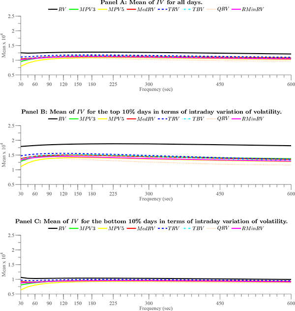
We provide signature plots for the mean of each pre-averaged estimator of IV as a function of pre-averaging window size matching the sampling frequency (measured in seconds on the x-axis). Panel A plots the mean across all days. Panel B plots the mean across the top 10% days with respect to intraday variation in volatility. Panel C plots the mean across the bottom 10% days with respect to intraday variation in volatility. Intraday variation in volatility is measured by the V oV measure of volatility of volatility described in Section 6.
Data for Figure 5, Panel A: Mean (x 10^4) of IV For All Days
| Frequency (sec) | RV | MPV3 | MPV5 | MedRV | TRV | TBV | QRV | RMinRV |
|---|---|---|---|---|---|---|---|---|
| 30 | 1.251884583 | 0.958551049 | 0.794837137 | 1.050386554 | 1.108841871 | 1.021009036 | 1.050368286 | 1.011301061 |
| 45 | 1.240427788 | 1.015900953 | 0.905233404 | 1.061270742 | 1.116815868 | 1.051249276 | 1.048687263 | 1.0373291 |
| 60 | 1.245180899 | 1.054981825 | 0.970684965 | 1.081438625 | 1.133234936 | 1.078672784 | 1.057689488 | 1.061914918 |
| 75 | 1.252532164 | 1.082041457 | 1.012162791 | 1.100383368 | 1.147583156 | 1.099965949 | 1.065566161 | 1.081304584 |
| 90 | 1.25903186 | 1.101218647 | 1.039562458 | 1.114048418 | 1.158290921 | 1.114885241 | 1.070461982 | 1.095103259 |
| 120 | 1.2680465 | 1.123873114 | 1.070614799 | 1.132082931 | 1.171693346 | 1.132898599 | 1.072164372 | 1.111266901 |
| 150 | 1.272537466 | 1.134766757 | 1.084669682 | 1.139628165 | 1.177157883 | 1.140914767 | 1.067865734 | 1.117304693 |
| 180 | 1.274062492 | 1.139652713 | 1.091031384 | 1.142783284 | 1.178085612 | 1.142917754 | 1.061406503 | 1.118967025 |
| 225 | 1.272713985 | 1.139434501 | 1.092115561 | 1.14171477 | 1.174619809 | 1.140426198 | 1.048426017 | 1.11616094 |
| 300 | 1.264602949 | 1.130578613 | 1.083323964 | 1.131335189 | 1.160997601 | 1.126193892 | 1.026726498 | 1.103180975 |
| 450 | 1.238713518 | 1.103201283 | 1.053442306 | 1.102535903 | 1.127560864 | 1.087865084 | 0.989489818 | 1.071352117 |
| 600 | 1.212630859 | 1.07727044 | 1.024563562 | 1.075803988 | 1.098021964 | 1.052253891 | 0.968514422 | 1.0424071 |
Data for Figure 5, Panel B: Mean (x 10^4) of IV for the Top 10% Days in Terms of Intraday Variation of Volatility
| Frequency (sec) | RV | MPV3 | MPV5 | MedRV | TRV | TBV | QRV | RMinRV |
|---|---|---|---|---|---|---|---|---|
| 30 | 1.791308526 | 1.28832395 | 1.109858253 | 1.379652254 | 1.474582587 | 1.357855589 | 1.385674883 | 1.332443208 |
| 45 | 1.808395937 | 1.36966899 | 1.233389255 | 1.425229399 | 1.509050078 | 1.417710152 | 1.393857513 | 1.382516833 |
| 60 | 1.825636059 | 1.425067337 | 1.312078123 | 1.4585819 | 1.531895237 | 1.459318265 | 1.399377542 | 1.416900981 |
| 75 | 1.839286468 | 1.455663491 | 1.356757493 | 1.479419676 | 1.544269167 | 1.485873165 | 1.399885101 | 1.435761221 |
| 90 | 1.849269302 | 1.476240167 | 1.382050553 | 1.489296872 | 1.551836014 | 1.498829328 | 1.394505684 | 1.445393125 |
| 120 | 1.864338254 | 1.496091624 | 1.409454643 | 1.500399676 | 1.557248506 | 1.513628464 | 1.379177435 | 1.451926121 |
| 150 | 1.873893928 | 1.501409369 | 1.412835636 | 1.494248369 | 1.551952373 | 1.515325927 | 1.359331111 | 1.442332755 |
| 180 | 1.879515242 | 1.500622253 | 1.411383763 | 1.489619882 | 1.541556205 | 1.507034983 | 1.34193356 | 1.433314958 |
| 225 | 1.88292431 | 1.482199717 | 1.395997252 | 1.472438277 | 1.523515411 | 1.488578865 | 1.307610203 | 1.413496149 |
| 300 | 1.878663654 | 1.451867085 | 1.367440507 | 1.439637528 | 1.48313302 | 1.450070889 | 1.262404469 | 1.380603429 |
| 450 | 1.849924495 | 1.40630547 | 1.315660776 | 1.388536935 | 1.411109831 | 1.376042037 | 1.188980342 | 1.332148809 |
| 600 | 1.816754692 | 1.374067481 | 1.277159656 | 1.352763392 | 1.358194549 | 1.312988669 | 1.158099485 | 1.292541786 |
Data for Figure 5, Panel C: Mean (x 10^4) of IV for the Bottom 10% Days in Terms of Intraday Variation of Volatility
| Frequency (sec) | RV | MPV3 | MPV5 | MedRV | TRV | TBV | QRV | RMinRV |
|---|---|---|---|---|---|---|---|---|
| 30 | 1.064453186 | 0.808401941 | 0.63944721 | 0.923949842 | 0.968292186 | 0.880766271 | 0.930248805 | 0.876132417 |
| 45 | 1.032398946 | 0.85268469 | 0.744624692 | 0.906240363 | 0.952690049 | 0.891556499 | 0.909594605 | 0.883767604 |
| 60 | 1.026416935 | 0.882320488 | 0.804331714 | 0.91103945 | 0.957266407 | 0.906735756 | 0.911336901 | 0.897698073 |
| 75 | 1.028838898 | 0.905278379 | 0.843978628 | 0.923324475 | 0.967302336 | 0.922738742 | 0.920267602 | 0.912815121 |
| 90 | 1.0317358 | 0.921134382 | 0.870431614 | 0.933955688 | 0.974988916 | 0.933904004 | 0.924939003 | 0.924588799 |
| 120 | 1.036663109 | 0.941568242 | 0.902112339 | 0.948157048 | 0.986868364 | 0.948836198 | 0.931165084 | 0.940793712 |
| 150 | 1.038761362 | 0.95147137 | 0.917081798 | 0.956034978 | 0.992809489 | 0.956542772 | 0.931747254 | 0.947183656 |
| 180 | 1.038800034 | 0.957645367 | 0.925342794 | 0.96098025 | 0.995418964 | 0.960751063 | 0.92995458 | 0.951781305 |
| 225 | 1.037083671 | 0.961733579 | 0.932318162 | 0.96456372 | 0.995250643 | 0.961887961 | 0.923971107 | 0.954821329 |
| 300 | 1.031355213 | 0.959019955 | 0.931353631 | 0.961688764 | 0.989846395 | 0.955404304 | 0.912235765 | 0.950804045 |
| 450 | 1.013458778 | 0.947926465 | 0.918609213 | 0.947701279 | 0.972184923 | 0.934043604 | 0.885822933 | 0.933863524 |
| 600 | 0.99400008 | 0.929011307 | 0.900639918 | 0.928322869 | 0.951593867 | 0.909432162 | 0.870820867 | 0.913544516 |
Figure 6: Average Estimates of √IQ Across the DJ30 Stocks Between January 1, 2005 and May 31, 2007
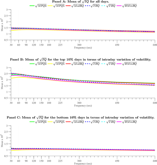
We provide signature plots for the mean of each pre-averaged estimator of √IQ as a function of pre-averaging window size matching the sampling frequency (measured in seconds on the x-axis). Panel A plots the mean across all days. Panel B plots the mean across the top 10% days with respect to intraday variation in volatility. Panel C plots the mean across the bottom 10% days with respect to intraday variation in volatility. Intraday variation in volatility is measured by the V oV measure of volatility of volatility described in Section 6.
Data for Figure 6, Panel A: Mean (x 10^4) of sqrt(IQ) For All Days
| Frequency (sec) | sqrt(MPQ3) | sqrt(MPQ5) | sqrt(MedRQ) | sqrt(TRQ) | sqrt(TBQ) | sqrt(RMinRQ) |
|---|---|---|---|---|---|---|
| 30 | 1.442376695 | 1.271094357 | 1.50213521 | 1.504948667 | 1.444731101 | 1.407577956 |
| 45 | 1.444610388 | 1.307127859 | 1.485826066 | 1.49324215 | 1.448247294 | 1.408467014 |
| 60 | 1.452406498 | 1.331527593 | 1.480005654 | 1.489189791 | 1.454337115 | 1.412584774 |
| 75 | 1.456050694 | 1.345995836 | 1.480198261 | 1.483994876 | 1.459416869 | 1.414846807 |
| 90 | 1.458908677 | 1.353859658 | 1.474429668 | 1.477593141 | 1.459394652 | 1.413456046 |
| 120 | 1.451633657 | 1.35302455 | 1.462847805 | 1.460877787 | 1.450830461 | 1.402183023 |
| 150 | 1.437650566 | 1.341985334 | 1.443333611 | 1.440123597 | 1.435805524 | 1.383074686 |
| 180 | 1.420556028 | 1.326830613 | 1.423955646 | 1.419035361 | 1.417242032 | 1.363768566 |
| 225 | 1.390721105 | 1.299967575 | 1.395086586 | 1.387299716 | 1.388898641 | 1.33589928 |
| 300 | 1.345483541 | 1.256945533 | 1.347919167 | 1.335407628 | 1.337876703 | 1.288199082 |
| 450 | 1.269947515 | 1.179696407 | 1.271543387 | 1.250640528 | 1.249169191 | 1.211242228 |
| 600 | 1.214550642 | 1.121440971 | 1.215479447 | 1.188109624 | 1.18259545 | 1.153606787 |
Data for Figure 6, Panel B: Mean (x 10^4) of sqrt(IQ) For the Top 10% Days in Terms of Intraday Variation of Volatility
| Frequency (sec) | sqrt(MPQ3) | sqrt(MPQ5) | sqrt(MedRQ) | sqrt(TRQ) | sqrt(TBQ) | sqrt(RMinRQ) |
|---|---|---|---|---|---|---|
| 30 | 2.414740215 | 2.131835896 | 2.529935902 | 2.546686961 | 2.468925337 | 2.366451326 |
| 45 | 2.420568695 | 2.176680926 | 2.50887977 | 2.511243842 | 2.473547662 | 2.362449527 |
| 60 | 2.429457688 | 2.209532142 | 2.475168122 | 2.456280306 | 2.456847426 | 2.339163034 |
| 75 | 2.399010398 | 2.200776601 | 2.443093202 | 2.39928646 | 2.43300215 | 2.303167315 |
| 90 | 2.378259469 | 2.181394988 | 2.389039727 | 2.350623616 | 2.389946912 | 2.262629619 |
| 120 | 2.312344377 | 2.125137108 | 2.312115428 | 2.264330651 | 2.320651894 | 2.180939663 |
| 150 | 2.247092381 | 2.057203767 | 2.221097096 | 2.180940004 | 2.252617282 | 2.091878004 |
| 180 | 2.186278118 | 1.997357848 | 2.156025381 | 2.107443178 | 2.179336298 | 2.022320003 |
| 225 | 2.074451936 | 1.896801638 | 2.057565038 | 2.010745134 | 2.080771114 | 1.92552261 |
| 300 | 1.949026038 | 1.782661999 | 1.932553109 | 1.867569482 | 1.939285464 | 1.806456873 |
| 450 | 1.801909048 | 1.629143347 | 1.779328859 | 1.668547958 | 1.734506235 | 1.660187785 |
| 600 | 1.717754237 | 1.535824664 | 1.691467327 | 1.54234234 | 1.592346649 | 1.570102974 |
Data for Figure 6, Panel C: Mean (x 10^4) of sqrt(IQ) For the Bottom 10% Days in Terms of Intraday Variation of Volatility
| Frequency (sec) | sqrt(MPQ3) | sqrt(MPQ5) | sqrt(MedRQ) | sqrt(TRQ) | sqrt(TBQ) | sqrt(RMinRQ) |
|---|---|---|---|---|---|---|
| 30 | 1.090740691 | 0.946622293 | 1.139040823 | 1.141013853 | 1.089748749 | 1.061179101 |
| 45 | 1.07110994 | 0.965648165 | 1.103721548 | 1.119139565 | 1.072358894 | 1.047801578 |
| 60 | 1.071849801 | 0.982760021 | 1.096716227 | 1.118325466 | 1.074127235 | 1.049474111 |
| 75 | 1.077733714 | 0.998254846 | 1.09861362 | 1.121553326 | 1.082446844 | 1.056759469 |
| 90 | 1.08192871 | 1.009411932 | 1.100501898 | 1.122008225 | 1.085647361 | 1.060421738 |
| 120 | 1.085857229 | 1.021904627 | 1.096876864 | 1.122263116 | 1.087921338 | 1.064571332 |
| 150 | 1.083122395 | 1.024420811 | 1.091681302 | 1.117110224 | 1.086362856 | 1.060617879 |
| 180 | 1.080635847 | 1.024169381 | 1.087006936 | 1.111299634 | 1.084712838 | 1.058277823 |
| 225 | 1.072625041 | 1.020861563 | 1.079842314 | 1.098481188 | 1.074911694 | 1.054189024 |
| 300 | 1.053372014 | 1.00387738 | 1.058810539 | 1.075018636 | 1.052173614 | 1.033618461 |
| 450 | 1.022146184 | 0.972097321 | 1.022660943 | 1.033864489 | 1.009762647 | 0.997645627 |
| 600 | 0.984909963 | 0.937265354 | 0.987750397 | 0.995117265 | 0.970799129 | 0.959921452 |
Figure 7: Average Estimates of √IQ/IV Across the DJ30 Stocks Between January 1, 2005 and May 31, 2007
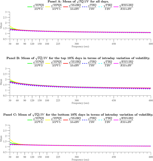
We provide signature plots for the mean of each pre-averaged estimator of √IQ/IV as a function of pre-averaging window size matching the sampling frequency (measured in seconds on the x-axis). Panel A plots the mean across all days. Panel B plots the mean across the top 10% days with respect to intraday variation in volatility. Panel C plots the mean across the bottom 10% days with respect to intraday variation in volatility. Intraday variation in volatility is measured by the V oV measure of volatility of volatility described in Section 6.
Data for Table 7, Panel A: Mean of sqrt(IQ)/IV For All Days
| Frequency (sec) | sqrt(MPQ3)/MPV3 | sqrt(MPQ5)/MPV5 | sqrt(MedRQ)/MedRV | sqrt(TRQ)/TRV | sqrt(TBQ)/TBV | sqrt(RMinRQ)/RMinRV |
|---|---|---|---|---|---|---|
| 30 | 1.507107116 | 1.688520391 | 1.404610311 | 1.333432815 | 1.39682524 | 1.372414188 |
| 45 | 1.415373352 | 1.48084126 | 1.377412284 | 1.315776639 | 1.358444536 | 1.339494557 |
| 60 | 1.365901129 | 1.384631033 | 1.350467704 | 1.29561673 | 1.330886944 | 1.313878287 |
| 75 | 1.333151781 | 1.332468752 | 1.328276659 | 1.276388978 | 1.310060192 | 1.292631281 |
| 90 | 1.309737645 | 1.29804305 | 1.30761283 | 1.25971896 | 1.292462826 | 1.275175229 |
| 120 | 1.274756732 | 1.25391734 | 1.275058403 | 1.231385714 | 1.263612388 | 1.245655383 |
| 150 | 1.249296936 | 1.224467131 | 1.249958514 | 1.208625869 | 1.241402007 | 1.222468807 |
| 180 | 1.228192509 | 1.201834695 | 1.22944161 | 1.190278298 | 1.223588791 | 1.203707929 |
| 225 | 1.203203523 | 1.176295435 | 1.205695507 | 1.167386557 | 1.201719466 | 1.181676008 |
| 300 | 1.173216794 | 1.145827553 | 1.176052292 | 1.138743558 | 1.173502872 | 1.154103509 |
| 450 | 1.134413428 | 1.107867389 | 1.1386597 | 1.101003192 | 1.136386898 | 1.118946506 |
| 600 | 1.11122577 | 1.083654651 | 1.115551977 | 1.076910652 | 1.114104639 | 1.096331805 |
Data for Table 7, Panel B: Mean of sqrt(IQ)/IV for the Top 10% Days in Terms of Intraday Variation of Volatility
| Frequency (sec) | sqrt(MPQ3)/MPV3 | sqrt(MPQ5)/MPV5 | sqrt(MedRQ)/MedRV | sqrt(TRQ)/TRV | sqrt(TBQ)/TBV | sqrt(RMinRQ)/RMinRV |
|---|---|---|---|---|---|---|
| 30 | 1.869772906 | 1.996228824 | 1.796450552 | 1.696402124 | 1.792326917 | 1.749964552 |
| 45 | 1.758004101 | 1.805429889 | 1.723958424 | 1.632565288 | 1.71478982 | 1.682568868 |
| 60 | 1.687659347 | 1.697808089 | 1.665577579 | 1.572967575 | 1.652188984 | 1.625985966 |
| 75 | 1.627424848 | 1.620863016 | 1.619109269 | 1.523349664 | 1.603359539 | 1.576199203 |
| 90 | 1.582478584 | 1.564781002 | 1.573784151 | 1.485077037 | 1.560275903 | 1.536602538 |
| 120 | 1.509960938 | 1.480947096 | 1.504130427 | 1.421401529 | 1.493874943 | 1.466579861 |
| 150 | 1.455961758 | 1.421286795 | 1.450322205 | 1.372759061 | 1.446281291 | 1.411986319 |
| 180 | 1.41476323 | 1.373692593 | 1.411000922 | 1.333901413 | 1.406450929 | 1.371972336 |
| 225 | 1.361373786 | 1.321218166 | 1.359959206 | 1.288107781 | 1.35865779 | 1.322928517 |
| 300 | 1.302423076 | 1.261113023 | 1.299854272 | 1.232724758 | 1.301405497 | 1.268472521 |
| 450 | 1.233709268 | 1.194729351 | 1.236934173 | 1.162867292 | 1.225713283 | 1.202619253 |
| 600 | 1.199779429 | 1.157911717 | 1.19962003 | 1.120995303 | 1.182343855 | 1.170356688 |
Data for Table 7, Panel C: Mean of sqrt(IQ)/IV for the Bottom 10% Days in Terms of Intraday Variation of Volatility
| Frequency (sec) | sqrt(MPQ3)/MPV3 | sqrt(MPQ5)/MPV5 | sqrt(MedRQ)/MedRV | sqrt(TRQ)/TRV | sqrt(TBQ)/TBV | sqrt(RMinRQ)/RMinRV |
|---|---|---|---|---|---|---|
| 30 | 1.390598436 | 1.66766297 | 1.23369788 | 1.180117752 | 1.248479554 | 1.218386657 |
| 45 | 1.289474933 | 1.400654313 | 1.228630236 | 1.181470229 | 1.216147175 | 1.198347103 |
| 60 | 1.240935776 | 1.284651078 | 1.217473453 | 1.177749366 | 1.200256028 | 1.183473185 |
| 75 | 1.214108691 | 1.229014611 | 1.205639107 | 1.171032638 | 1.190426406 | 1.173717965 |
| 90 | 1.197194467 | 1.197478017 | 1.195587597 | 1.162899062 | 1.18087963 | 1.164091418 |
| 120 | 1.172654296 | 1.161143029 | 1.174362496 | 1.148153688 | 1.163542539 | 1.147244041 |
| 150 | 1.155875825 | 1.139176304 | 1.15951379 | 1.134994194 | 1.150328581 | 1.135334708 |
| 180 | 1.143499694 | 1.124863049 | 1.145710064 | 1.125046599 | 1.141698091 | 1.125265033 |
| 225 | 1.126905012 | 1.107731499 | 1.132027953 | 1.110534543 | 1.12896346 | 1.114049269 |
| 300 | 1.108840734 | 1.088584894 | 1.113738203 | 1.091127156 | 1.111981387 | 1.095780815 |
| 450 | 1.083647284 | 1.065574076 | 1.085655326 | 1.066502664 | 1.088201084 | 1.074401761 |
| 600 | 1.066042116 | 1.047476475 | 1.069893784 | 1.049288809 | 1.074252286 | 1.057151672 |
7 Conclusion
We provide a first in-depth look at robust estimation of
integrated quarticity (IQ) based on high frequency data. The
sensitivity of many existing IQ estimators to pervasive data
irregularities inspires us to introduce a novel set of jump-robust
estimators that are defined in terms of order statistics of
suitable return functionals and generalize the existing nearest
neighbor truncation estimators of ADS (2012). This new class of
robust neighborhood truncation (RNT) estimators can be designed to
enhance the robustness properties vis-à-vis microstructure
noise features of the data as well as reducing the finite sample
sensitivity to outliers. The identical principle can more generally
be applied also to other consistent estimators to enhance jump- and
noise-robustness. We find that the novel RNT estimators outperform
existing estimators by a considerable margin in terms of finite
sample efficiency in estimating the key ratio of ![]() . This quantity is extremely useful for robust
inference regarding IV and for testing for price jumps.
. This quantity is extremely useful for robust
inference regarding IV and for testing for price jumps.
In the empirical implementation, we emphasize the importance of appropriate filtering for gross violations of the particular null hypothesis associated with a given estimation procedure. In particular, we apply a novel functional filtering scheme for local power variation estimators, which generalizes truncation of individual returns to truncation of return functionals and is easy to apply for a broad range of popular estimators. By invoking this approach at the level of the local power variation estimators, the threshold can be set very conservatively, thereby avoiding systematic biases arising from aggressive truncation and thus eliminating the need for ex-post bias correction. We also emphasize the use of pre-averaging based on a wide pre-averaging window. This allows for important robustness to extreme outliers, like the so-called bounce-backs, and it simplifies the associated distribution theory as the impact of noise vanishes asymptotically.
The unifying theme behind the new class of estimators, as well as the universal filtering procedure applied to them, is to operate directly on the functional space of local power variation estimates instead of restricting attention to the underlying individual returns. In fact, we may view the latter as a special case, arising from a block size of unity. Combining the functional filtering with the novel RNT class of estimators enables efficient inference in an extensive simulation design and generates supportive evidence from an empirical application using the Dow Jones 30 stocks. Overall, the study provides a set of new guidelines for the construction of practical robust and efficient estimation and inference regarding IV and IQ.
References
Andersen, T. G. and T. Bollerslev (1998). Answering the skeptics: Yes, standard volatility models do provide accurate forecasts. International Economic Review 39, 885-905.
Andersen, T. G., T. Bollerslev, and F. X. Diebold (2007). Roughing it up: Including jump components in the measurement, modeling, and forecasting of return volatility. Review of Economics and Statistics 89, 701-720.
Andersen, T. G., T. Bollerslev, and F. X. Diebold (2010). Parametric and Nonparametric Volatility Measurement. North Holland. In Handbook of Financial Econometrics, Volume 1 - Tools and Techniques; Yacine Ait-Sahalia, Lars P. Hansen, and Jose A. Scheinkman (Eds.).
Andersen, T. G., T. Bollerslev, F. X. Diebold, and P. Labys (2001). The distribution of realized exchange rate volatility. Journal of the American Statistical Association 96, 42-55.
Andersen, T. G., T. Bollerslev, F. X. Diebold, and P. Labys (2003). Modeling and forecasting realized volatility. Econometrica 71, 579-625.
Andersen, T. G., T. Bollerslev, and D. Dobrev (2007). No-arbitrage semi-martingale restrictions for continuous-time volatility models subject to leverage effects, jumps and i.i.d. noise: Theory and testable distributional implications. Journal of Econometrics 138, 125-180.
Andersen, T. G., D. P. Dobrev, and E. Schaumburg (2008). Duration based volatility estimation. Manuscript, Northwestern University.
Andersen, T. G., D. P. Dobrev, and E. Schaumburg (2011). A functional filtering and neighborhood truncation approach to integrated quarticity estimation. NBER Working Paper 17152.
Andersen, T. G., D. P. Dobrev, and E. Schaumburg (2012). Jump-robust volatility estimation using nearest neighbor truncation. Journal of Econometrics 169, 75-93.
Back, K. (1991). Asset pricing for general processes. Journal of Mathematical Economics 20, 371-395.
Bandi, F. M. and J. R. Russell (2008). Microstructure noise, realized variance, and optimal sampling. Review of Economic Studies 75, 339-369.
Barndorff-Nielsen, O. E., S. E. Graversen, J. Jacod, M. Podolskij, and N. Shephard (2006). A central limit theorem for realized power and bipower variations of continuous semimartingales. in From stochastic calculus to mathematical finance : the Shiryaev Festschrift, Springer Verlag.
Barndorff-Nielsen, O. E., S. E. Graversen, J. Jacod, and N. Shephard (2006). Limit theorems for bipower variation in financial econometrics. Econometric Theory 22, 677-719.
Barndorff-Nielsen, O. E., P. R. Hansen, A. Lunde, and N. Shephard (2008). Designing realized kernels to measure the ex post variation of equity prices in the presence of noise. Econometrica 76, 1481-1536.
Barndorff-Nielsen, O. E., P. R. Hansen, A. Lunde, and N. Shephard (2009). Realised kernels in practice: Trades and quotes. Econometrics Journal 12, C1-C32.
Barndorff-Nielsen, O. E. and N. Shephard (2002). Estimating quadratic variation using realized variance. Journal of Applied Econometrics 17, 457-477.
Barndorff-Nielsen, O. E. and N. Shephard (2004a). Econometric analysis of realized covariation: High frequency based covariance, regression, and correlation in financial economics. Econometrica 72, 885-925.
Barndorff-Nielsen, O. E. and N. Shephard (2004b). Power and bipower variation with stochastic volatility and jumps. Journal of Financial Econometrics 2, 1-37.
Barndorff-Nielsen, O. E. and N. Shephard (2006). Econometrics of testing for jumps in financial economics using bipower variation. Journal of Financial Econometrics 4, 1-30.
Barndorff-Nielsen, O. E., N. Shephard, and M. Winkel (2006). Limit theorems for multipower variation in the presence of jumps. Stochastic Processes and Their Applications 116, 796-806.
Christensen, K., R. Oomen, and M. Podolskij (2008). Realized quantile-based estimation of integrated variance. Working paper; CREATES, University of Aarhus, Denmark.
Christensen, K., R. Oomen, and M. Podolskij (2010). Realized quantile-based estimation of integrated variance. Journal of Econometrics 159, 74-98.
Corsi, F., D. Pirino, and R. Renò (2010). Threshold bipower variation and the impact of jumps on volatility forecasting. Journal of Econometrics 159, 276-288.
Hasbrouck, J. (1999). The dynamics of discrete bid and ask quotes. Journal of Finance 54, 2109-2142.
Hautsch, N. and M. Podolskij (2010). Pre-averaging based estimation of quadratic variation in the presence of noise and jumps: Theory, implementation, and empirical evidence. Journal of Business and Economic Statistics forthcoming.
Hsieh, D. A. (1991). Chaos and nonlinear dynamics: Applications to financial markets. Journal of Finance 46, 1839-1878.
Huang, X. and G. Tauchen (2005). The relative contribution of jumps to total price variance. Journal of Financial Econometrics 3, 456-499.
Jacod, J., Y. Li, P. Mykland, M. Podolskij, and M. Vetter (2009). Mirostructure noise in the continuous case: the pre-averaging approach. Stochastic Processes and Their Applications 26, 2803-2831.
Jacod, J. and P. Protter (1998). Asymptotic error distributions for the euler method for stochastic differential equations. Annals of Probability 26, 267-307.
Jacod, J. and A. N. Shiryaev (2003). Limit theorems for stochastic processes (2nd ed.). Grundlehren der mathematischen Wissenschaften. Berlin; New York: Springer.
Jiang, G. J. and R. C. Oomen (2008). Testing for jumps when asset prices are observed with noise - a “swap variance” approach. Journal of Econometrics 144, 352-370.
Mancini, C. (2009). Non-parametric threshold estimation for models with stochastic diffusion coefficient and jumps. Scandinavian Journal of Statistics 36, 270-296.
Mykland, P. A. and L. Zhang (2009). Inference for continuous semimartingales observed at high frequency. Econometrica 77, 1403-1445.
Podolskij, M. and M. Vetter (2009a). Bipower-type estimation in a noisy diffusion setting. Stochastic Processes and Their Applications 119, 2803-2831.
Podolskij, M. and M. Vetter (2009b). Estimation of volatility functionals in the simultaneous presence of microstructure noise and jumps. Bernoulli 15, 634-658.
Schwert, G. W. (1989). Why does stock market volatility change over time? The Journal of Finance 44, 1115-1153.
Zhang, L., P. A. Mykland, and Y. Ait-Sahalia (2005). A tale of two time scales: Determining integrated volatility with noisy high-frequency data. Journal of the American Statistical Association 100, 1394-1411.
Zhou, B. (1996). High-frequency data and volatility in foreign-exchange rates. Journal of Business and Economic Statistics 14, 45-52.
A Proofs of Propositions
This appendix
provides proofs of Proposition 1 and related results for the
general case of estimating the integrated power variation of order
![]() , where
, where ![]() is a positive and
even integer. The proofs are initially given for the MinPV and
MedPV type estimators and subsequently shown to extend to the RNT
estimators in Lemma 9 below.
is a positive and
even integer. The proofs are initially given for the MinPV and
MedPV type estimators and subsequently shown to extend to the RNT
estimators in Lemma 9 below.
The
(integrated) power variation, ![]() , is formally
defined as,
, is formally
defined as,
|
(3) |
Obviously,
![]() corresponds to the theoretical quantity
relevant for the
corresponds to the theoretical quantity
relevant for the ![]() and
and ![]() estimators while
estimators while ![]() refers to the integrated
variance underlying the
refers to the integrated
variance underlying the ![]() and
and ![]() estimators. The higher order integrated power variation
estimators are less commonly used but do appear in the recent
literature. For example,
estimators. The higher order integrated power variation
estimators are less commonly used but do appear in the recent
literature. For example, ![]() is required to assess the
(asymptotic) precision of integrated quarticity
estimators.
is required to assess the
(asymptotic) precision of integrated quarticity
estimators.
A.1 Basic Setting
Let ![]() be the log price process following a Brownian
semimartingale
be the log price process following a Brownian
semimartingale
|
(4) |
where ![]() is a locally bounded and predictable process and
is a locally bounded and predictable process and
![]() is adapted, cadlag and bounded away
from zero. Without loss of generality, we further assume that the
functions
is adapted, cadlag and bounded away
from zero. Without loss of generality, we further assume that the
functions
![]() are uniformly bounded and
are uniformly bounded and
![]() a.s.30 The extension allowing for finite
activity jumps in
a.s.30 The extension allowing for finite
activity jumps in ![]() is dealt with Section A.6 below.
is dealt with Section A.6 below.
When discussing central limit theorems (CLTs) we require in addition that the volatility process follows a generalized Itô process:
|
where ![]() is locally bounded and predictable and
is locally bounded and predictable and
![]() are cadlag and
the Brownian motions
are cadlag and
the Brownian motions ![]() are uncorrelated. We
impose, without loss of generality, that the functions
are uncorrelated. We
impose, without loss of generality, that the functions
![]() and
and
![]() are uniformly bounded as well as
are uniformly bounded as well as
![]() and
and
![]() a.s. We
further note that, when the volatility process
a.s. We
further note that, when the volatility process
![]() satisfies Assumption
A1, then the power variation process,
satisfies Assumption
A1, then the power variation process,
![]() , also conforms to
this general characterization.
, also conforms to
this general characterization.
We assume
![]() is observed at
is observed at ![]() evenly
spaced time points spanning the interval
evenly
spaced time points spanning the interval ![]() .
Below, we denote these observations by
.
Below, we denote these observations by ![]() ,
,
![]() , and the associated log-returns
by
, and the associated log-returns
by
![]() ,
,
![]() . The proofs involve sequences
of standardized return observations and corresponding approximating
sequences for which volatility is fixed across one or more returns.
Hence, we introduce non-overlapping blocks of
. The proofs involve sequences
of standardized return observations and corresponding approximating
sequences for which volatility is fixed across one or more returns.
Hence, we introduce non-overlapping blocks of ![]() returns for which the volatility process is
constant. We assume we have
returns for which the volatility process is
constant. We assume we have ![]() such blocks in
the sample. Consequently, we define the
quantities,
such blocks in
the sample. Consequently, we define the
quantities,
| (5) | |||
| (6) |
where
![]() indicates the integer
part of an expression. Hence, for each of the
indicates the integer
part of an expression. Hence, for each of the ![]() return blocks, corresponding to
return blocks, corresponding to
![]() , the volatility remains fixed
at the value it attains at the beginning of the
block.
, the volatility remains fixed
at the value it attains at the beginning of the
block.
A.2 The Min and Med Power Variation Estimators
Let ![]() be a fixed positive even integer and let
be a fixed positive even integer and let
![]() be
given by,
be
given by,
| (7) | |||
For example, we
have
![]() and
and
![]() .
.
Similarly, we
define the median-based function
![]() and scaling factors,
and scaling factors,
In this case,
![]() and
and
![]() .
.
For any even
positive integer, ![]() , we define the nearest
neighbor truncation estimators of the
, we define the nearest
neighbor truncation estimators of the ![]() 'th order
power variation by,
'th order
power variation by,
| MinPV |
|
|
| MedPV |
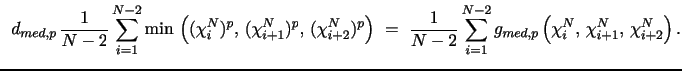
|
For the cases
of primary interest, i.e., ![]() and
and ![]() , these estimators are identical to the
, these estimators are identical to the ![]() and
and ![]() estimators introduced in Section
2.1. Specifically, we have
estimators introduced in Section
2.1. Specifically, we have
| MinPV |
| MinPV |
A.3 Additional Notation and Preliminary Results
We provide a
detailed proof of the results in Propositions 1 and 2 concerning
the
MinPV![]() estimator. The proofs for
MedPV
estimator. The proofs for
MedPV![]() may be derived similarly. Moreover, we
henceforth consider a fixed even, positive integer,
may be derived similarly. Moreover, we
henceforth consider a fixed even, positive integer, ![]() ,
so the
,
so the
![]() function is uniquely
defined. We refer to it simply as
function is uniquely
defined. We refer to it simply as ![]() below.
below.
First, we
observe that, for any bivariate vectors,
![]() and
and
![]() , we have the following
useful bound,
, we have the following
useful bound,
| (8) |
and furthermore
that, except on the null set
![]() , we
have
, we
have
![$\displaystyle \lim_{{\varepsilon\rightarrow0}} \,\, \frac{1}{\varepsilon} \,\, \left[\,\min(\,a_1^{p},\,a_2^{p} \, + \, \varepsilon \, z) \, \, - \, \min(\,a_1^{p},\, a_2^{p}\,)\,\right] \,\,\, = \,\,\, \left\{ \begin{array}{ll} z&\text{if } \,\,\,\,\, \vert a_2\vert \, < \, \vert a_1\vert \\ 0& \text{if } \,\,\,\,\, \vert a_2\vert \, > \, \vert a_1\vert \end{array}\right.$](img405.gif)
|
(9) |
The proofs of Propositions 1 and 2 revolve around the sequences,
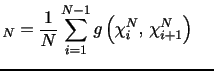 and
and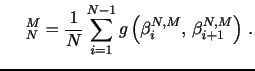
|
Since
MinPV![]() the
the
![]() sequence is asymptotically equivalent to
our
sequence is asymptotically equivalent to
our ![]() estimator, while
estimator, while ![]() is an approximating sequence as, for large
is an approximating sequence as, for large
![]() .
.
For any
adapted, integrable, ![]() -dimensional cadlag process,
-dimensional cadlag process,
![]() , and for
, and for
![]() , we define the
expectation conditional on information at time
, we define the
expectation conditional on information at time
![]() :
:
| (10) |
A useful implication of our ability to focus on the case with uniformly bounded drift and volatility functions is that, using the Burkholder-Davis-Grundy inequalities, we have,
| (11) |
where
![]() and
and ![]() denotes a generic positive constant which we (with slight abuse of
notation) allow to take on disparate values in different
places.
denotes a generic positive constant which we (with slight abuse of
notation) allow to take on disparate values in different
places.
We decompose
our estimators for the power variation, ![]() , into a
sum of conditional expectations and the associated martingale
difference sequences:
, into a
sum of conditional expectations and the associated martingale
difference sequences:
![]() and
and
![]() where,
where,
![$\displaystyle \V_{1N}=\frac{1}{N}\sum_{i=1}^{N-1} E_{i-1} \left[g \left( \chi_{i}^N,\chi_{i+1}^N \right) \right], \,\,\,\,\,\,\,\,\,\, \V_{2N}=$](img425.gif)
|
![$\displaystyle \frac{1}{N}\sum_{i=1}^{N-1} \left\{ g(\chi_{i}^N,\chi_{i+1}^N) - E_{i-1} \left[g(\chi_{i}^N,\chi_{i+1}^N) \right]\right\}$](img426.gif)
|
![$\displaystyle \U_{1N}^M=\frac{1}{N}\sum_{i=1}^{N-1} E_{\lfloor\frac{i-1}{M}\rfloor M} \left[ g \left (\beta_i^{N,M},\beta_{i+1}^{N,M} \right) \right], \,\,\, \U_{2N}^M=$](img427.gif)
|
![$\displaystyle \frac{1}{N}\sum_{i=1}^{N-1} \left\{ g(\beta_{i}^{N,M}, \beta_{i+1}^{N,M}) - E_{\lfloor\frac{i-1}{M}\rfloor M} \left[ g(\beta_{i}^{N,M}, \beta_{i+1}^{N,M}) \right] \right\}.$](img428.gif)
|
When
![]() we will use the shorthand
we will use the shorthand
![]() and similarly for the individual pieces
and similarly for the individual pieces
![]() and
and ![]() . These
definitions allow us to decompose the main
estimator:
. These
definitions allow us to decompose the main
estimator:
| (12) |
Consistency of
![]() can then be obtained by showing
consistency of the estimator applied to the approximating Brownian
path with piecewise constant volatility (
can then be obtained by showing
consistency of the estimator applied to the approximating Brownian
path with piecewise constant volatility (
![]() ) and then showing
that the difference
) and then showing
that the difference
![]() (the last two terms in (12)
above) is asymptotically negligible. This is what we do in Section A.4 below. To prove a CLT, we exploit a different decomposition
(similar to Mykland and Zhang (2007)), in which we show the CLT for
our estimator applied to an approximating Brownian motion for which
volatility is piecewise constant over blocks of length
(the last two terms in (12)
above) is asymptotically negligible. This is what we do in Section A.4 below. To prove a CLT, we exploit a different decomposition
(similar to Mykland and Zhang (2007)), in which we show the CLT for
our estimator applied to an approximating Brownian motion for which
volatility is piecewise constant over blocks of length ![]() . We then proceed to show that the difference between the
original estimator and the estimator applied to the approximating
process is negligible. This analysis is carried out in Section A.5 based on the
decomposition:
. We then proceed to show that the difference between the
original estimator and the estimator applied to the approximating
process is negligible. This analysis is carried out in Section A.5 based on the
decomposition:
| (13) |
A.4 Proposition 2: Consistency
We proceed by
analyzing equation (12) term by term
through a series of lemmas. For brevity, we focus on the features
that are specific to our estimator, while referring to proofs in
the extant literature when feasible. This also serves to highlight
the underlying structural similarities between our ![]() measure and previously proposed power variation
estimators and, in particular,
measure and previously proposed power variation
estimators and, in particular, ![]() and
and ![]() estimators.
estimators.
Lemma 2 Under the maintained assumptions we have,
| (14) |
Moreover, if Assumption (A1) holds we obtain,
| (15) |
Proof. First, note that
so we may write
![$\displaystyle \, \frac{1}{N}\sum_{i=1}^{N-1}\E_{i-1}\left[\,g\left (\beta_i^{N}, \beta_{i+1}^{N} \right)\, - \, g\left (\beta_i^{N}, \sqrt{N}\sigma_{\frac{i-1}{N}} \, \Delta_{i+1}^{N}B \, \right)\, \right] \, + \, \frac{1}{N} \sum_{i=1}^{N-1} \sigma^{p}_{\frac{i-1}{N}}$](img456.gif)
|
(16) |
The first sum in (16) tends to zero
in probability. To see this, note that the bound (8) implies the
following limit in ![]() -norm:
-norm:
![$\displaystyle \E\left\vert\, \frac{1}{N}\sum_{i=1}^{N-1}\E_{i-1}\left[g\left (\beta_i^{N}, \beta_{i+1}^{N} \right)-g\left (\beta_i^{N}, \sqrt{N}\sigma_{\frac{i-1}{N}}\Delta_{i+1}^{N}B \right)\right]\, \right\vert^{\,2} \,\, \leq \,\, \frac{C}{N} \,\, \E \left[ \, \sum_{i=1}^{N-1} \vert\sigma^{p}_{\frac{i}{N}} - \sigma^{p}_{\frac{i-1}{N}}\vert^{\,2} \, \right] \,\, \rightarrow \,\, 0$](img458.gif)
|
(17) |
where the convergence (17), and thus also
convergence in probability, follows from the fact that
![]() has finite quadratic
variation (since
has finite quadratic
variation (since
![]() is a cadlag semimartingale). In
addition, since
is a cadlag semimartingale). In
addition, since
![]() is uniformly
bounded and cadlag, the pointwise dominated convergence of
is uniformly
bounded and cadlag, the pointwise dominated convergence of
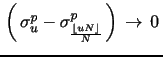 for
for
![]() follows and Lebesgue's
theorem yields
follows and Lebesgue's
theorem yields
![$\displaystyle \sum_{i=1}^{N-1} \left[ \, \int_{\frac{(i-1)}{N}}^{\frac{i}{N}} \left(\sigma_{u}^{p} -\sigma^{p}_{ \frac{(i-1)}{N}}\right)\,du \, \right] \, \overset{a.s.}{\rightarrow} \, 0$](img464.gif)
|
(18) |
Together (17) and (18) imply
![]() which establishes (14). To show
(15)
we need the stronger assumption (A1). Define the sequence of
independent standard normals
which establishes (14). To show
(15)
we need the stronger assumption (A1). Define the sequence of
independent standard normals
![]() , then
Assumption (A1) yields
, then
Assumption (A1) yields
![$\displaystyle \E_{i-1}\left[\,(\sigma^{\, p}_{\frac{i}{N}} - \sigma^{\, p}_{\frac{i-1}{N}}) \, Z_{i+1}^{p}\mathbf{1}_{\vert Z_{i+1}\vert<\vert Z_{i}\vert} \, \right] \, = \, \E_{i-1}\left[\,(\sigma^{\, p}_{\frac{i}{N}}-\sigma^{\, p}_{\frac{i-1}{N}})\, \varphi(Z_{i}) \, \right] \, = \, O_{P \,}(1/N)$](img467.gif)
|
(19) |
since![]() ce
is an even function of the Brownian path
ce
is an even function of the Brownian path
![]() . Now the
property (9) yields
. Now the
property (9) yields
| (20) |
This ensures that the first term in (16) is
asymptotically negligible, even when scaled up by ![]() . Hence, the remaining task is to show,
. Hence, the remaining task is to show,
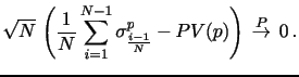
|
However, this is analogous to the common task of showing that
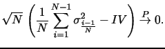
|
in the IV literature and the method of proof is, by now, well established; see, e.g., BNGJPS where the result is shown in a general setting (allowing for infinite activity jumps) of which the current framework is a special case. A more intuitive and detailed exposition is provided by Barndorff-Nielsen, Graversen, Jacod, and Shephard (2006), henceforth BNGJS.
Lemma 3 Under the maintained assumptions, we have
| (21) |
Proof. To simplify notation, define the martingale
difference sequence
![]() :
:
Note that
![]() , so applying the Cauchy-Schwartz inequality,
, so applying the Cauchy-Schwartz inequality,
![$\displaystyle \V\left[\frac{1}{N} \sum_{i=1}^N \eta_i^N\right] \, = \, \frac{1}{N} \, \E\left[ \, \frac{1}{N} \sum_{i=1}^N \left( (\eta_i^N)^2 \, + \, 2 \eta_i^N \eta_{i+1}^N \right) \, \right] \, \le \, \frac{C}{N} \, \E\left[ \, \frac{1}{N}\sum_{i=1}^N \E [ \, (\eta_i^N)^2\vert \mathcal{F}_{\frac{i-1}{N}} \,] \, \right] \, \le \, \frac{C}{N} \, \rightarrow \, 0 \,.$](img479.gif)
|
The ![]() convergence implies
.
convergence implies
. ![]()
![]() .
.
Lemma 4 Under the maintained assumptions, we have,
| (22) |
Under Assumption (A1), we obtain,
| (23) |
Proof. We must show,
![$\displaystyle V_{1N} - U_{1N} \, = \, \frac{1}{N} \sum_{i=1}^{N-1} \E_{i-1} \left[ \, \left( g(\chi_{i}^N,\,\chi_{i+1}^N) - g(\beta_{i}^N,\,\beta_{i+1}^N) \right) \, \right] \, \rightarrow \, 0 \,\,\,$](img485.gif) as
as |
(24) |
Using the bound (8), it follows that,
![$\displaystyle \,\,\,\, \frac{1}{N} \E\left[\, \sum_{i=1}^{N-1} \, \vert\,g(\chi_{i}^N\,,\chi_{i+1}^N) \, - \, g(\beta_{i}^{N }, \, \beta_{i+1}^{N})\,\vert \, \right]$](img488.gif)
|
|
![$\displaystyle \,\,\,\, \frac{C}{N} \,\, \E\left[\, \sum_{i=1}^N \, \left\vert \, (\chi_i^N)^p - (\beta_i^N)^p \, \right\vert \, \right] \,\, = \,\, \frac{C}{N} \,\, \sum_{i=1}^N \, \left( \, \E_{i-1} \left\vert \, h(\sqrt{N} \Delta_i^N Y) \, - \, \sigma_{\frac{i-1}{N}}^p \, \right\vert \, \right)$](img490.gif)
|
where we have defined the function
![]() . This formulation maps directly
into the setting of BNGJPS where the results of this lemma are
proven in a more general setting and for a generic
. This formulation maps directly
into the setting of BNGJPS where the results of this lemma are
proven in a more general setting and for a generic ![]() function subject to regularity conditions. In
particular, our
function subject to regularity conditions. In
particular, our ![]() function trivially satisfies the
continuous differentiability and polynomial growth conditions
necessary for the applicability of their analysis. An accessible,
albeit lengthy, account of the steps of the argument may be found
in BNGJS (2006, pp. 713-719). So while this proof is quite
involved, the above reformulation of the relevant inequalities, as
they arise within our specific setting, allows us to simply refer
to previously published work for the result.
function trivially satisfies the
continuous differentiability and polynomial growth conditions
necessary for the applicability of their analysis. An accessible,
albeit lengthy, account of the steps of the argument may be found
in BNGJS (2006, pp. 713-719). So while this proof is quite
involved, the above reformulation of the relevant inequalities, as
they arise within our specific setting, allows us to simply refer
to previously published work for the result. ![]()
Lemma 5 Under the maintained assumptions, we have,
| (25) |
Moreover, we may strengthen this result further to obtain,
| (26) |
Proof. In order to demonstrate the second result of the lemma, which obviously implies the first, we define,
and we must then prove that,
![$\displaystyle \sum_{i=1}^{N-1} \, \left( \, \xi_i^N - \E_{i-1} [ \, \xi_i^N \, ] \, \right) \,\, \overset{P}\rightarrow \,\, 0 \, .$](img498.gif)
|
This is a martingale difference sequence with respect to the
filtration
![]() , so it
suffices to show,
, so it
suffices to show,
![$\displaystyle \sum_{i=1}^{N-1} \, \E \left[ \, (\xi_i^N)^2 \, \right] \,\, = \,\, \E \left[ \, \sum_{i=1}^{N-1} \E_{i-1} \left[ \, (\xi_i^N)^2 \, \right] \, \right] \, \rightarrow \, 0 \,\,\,\,\,\,$](img500.gif) as
as |
Mimicking the type of steps undertaken in the proof of the previous
lemma, including application of the uniform bound on moments of
![]() and
and
![]() , we obtain,
, we obtain,
![$\displaystyle \sum_{i=1}^{N-1} \, \E \left[ \,(\xi_i^N)^2 \, \right] \,\,\,$](img504.gif)
|
![$\displaystyle \,\,\, \frac{1}{N} \,\, \E \left[ \, \sum_{i=1}^{N-1} \, \E_{i-1} \left\vert \, g( \, \chi_{i}^N, \, \chi_{i+1}^N) \, - \, g(\beta_i^N, \, \beta_{i+1}^N \, ) \, \right\vert^2 \, \right]$](img506.gif)
|
|
![$\displaystyle \,\, \frac{C}{N} \,\, \E \left[ \sum_{i=1}^{N} \E_{i-1} \left[ \, \left( \, h(\chi_i^N) - h(\beta_i^N) \, \right)^2 \, \right] \, \right] \, .$](img508.gif)
|
As for the previous lemma, our reformulation of the task maps the problem into the corresponding task in BNGJPS (2006) who prove a corresponding lemma in a more general setting. A detailed account of the requisite steps to complete this part of the proof may again be gleaned from BNGJS (2006, pp. 704-706).
Taken together, Lemma 2-3 and the first parts of Lemma 4-5 simply the consistency of our estimator under the minimal maintained assumptions. The second parts of Lemmas 4-5 are critical for the proof of the central limit theorem below.
A.5 Proposition 3: The CLT
Lemma 6 Under assumption (A1), we have
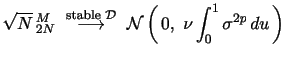
|
(27) |
where the constant
![]() for
for
![]() .
.
Proof. Consider splitting the ![]() scaled
return observations into
scaled
return observations into ![]() blocks, the
blocks, the
![]() of which is the vector
of which is the vector
![]() . The corresponding vector of observations from the approximating
Brownian motion where volatility is held constant over the block is
. The corresponding vector of observations from the approximating
Brownian motion where volatility is held constant over the block is
![]() . Next, define by
. Next, define by
![]() the block estimator of volatility:
the block estimator of volatility:
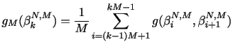
|
(28) |
We wish to apply Theorem IX.7.28 in Jacod and Shiryaev (2003) to
![]() . Defining the
martingale difference sequence
. Defining the
martingale difference sequence
 we can write
![$\displaystyle =\,\, \frac{1}{\sqrt{K}} \, \sum_{k=1}^{K} \psi_{k}^{N,M} \, + \, \frac{1}{\sqrt{N}} \, \sum_{k=1}^{K-1} \, \left(g(\,\beta_{kM}^{N,M},\,\beta_{kM+1}^{N,M}) \,-\, \E_{\frac{k-1}{K}}\left[g(\,\beta_{kM}^{N,M},\,\beta_{kM+1}^{N,M})\,\right]\,\right)$](img523.gif)
|
||
|
(29) |
The last equality follows from the fact that each term in the
second sum is centered and has bounded variance (given the uniform
bound on ![]() ). Thus the sum divided by
). Thus the sum divided by
![]() will tend to zero provided
will tend to zero provided
![]() .
.
We must now verify conditions (7.27)-(7.31) of Theorem IX.7.28.
First note that
![]() so that condition (7.27) is trivially satisfied. Condition (7.28)
follows from the fact that
so that condition (7.27) is trivially satisfied. Condition (7.28)
follows from the fact that
![$\displaystyle \frac{1}{K}\, \sum_{k=1}^{K} E\left[ \left\{ \, \sqrt{M} \left( \, g_M( \, \mathbf{\beta}_k^{M} \, ) \, - \, \frac{M-1}{M} \sigma_{\frac{(k-1)}{K}}^{\,p} \, \right) \, \right\}^{2} \, \vert \, \mathcal{F}_{\frac{k-1}{K}} \, \right] \, = \, \frac{\nu}{K} \, \sum_{k=1}^{K} \, \sigma^{2p}_{\frac{k-1}{K}} \, \overset{P}{\rightarrow} \, \nu \, \int_{0}^{1} \sigma^{2p}_{u}\,du$](img529.gif)
|
(30) |
where the convergence in probability (and in fact a.s.) is a
consequence of the volatility process being cadlag and uniformly
bounded. Next, we turn to condition (7.29). Let
 , then
![]() , which follows from the fact that the variables
, which follows from the fact that the variables
![]() are centered and that
are centered and that
![]() is an even function. Condition (7.30),
stating that
is an even function. Condition (7.30),
stating that
![$ E\left[(\psi_{k}^{N,M})^{2}\,\mathbf{1}_{\vert\psi_{k}^{N,M}\vert>\varepsilon}\right]\overset{P}{\rightarrow}0$](img534.gif) , follows straightforwardly from the fact that
, follows straightforwardly from the fact that ![]() is uniformly bounded.
is uniformly bounded.
Finally, let
![]() be a bounded
martingale orthogonal to
be a bounded
martingale orthogonal to ![]() (i.e. the covariation
(i.e. the covariation
![]() ). We want
to show that, for each block
). We want
to show that, for each block ![]() ,
,
![$ E[\psi_{k}^{N,M}\left(N_\frac{k}{K}-N_\frac{(k-1)}{K}\right)\vert\mathcal{F}_{\frac{k-1}{K}}]=0$](img540.gif) . For
. For
![]() consider the martingale
difference sequence
consider the martingale
difference sequence
![]() . By the martingale representation theorem,
. By the martingale representation theorem,
 for some predictable process
![]() . Therefore the processes
. Therefore the processes
![]() and
and
![]() are
orthogonal and the product,
are
orthogonal and the product,
![]() is again
a martingale which must then have mean zero. This verifies
condition (7.31) and Theorem IX.7.28 in Jacod and Shiryaev (2003)
states that as
is again
a martingale which must then have mean zero. This verifies
condition (7.31) and Theorem IX.7.28 in Jacod and Shiryaev (2003)
states that as ![]() (and hence
(and hence ![]() and
and
![]() ) tend to infinity:
) tend to infinity:
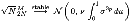
|
(31) |
Lemma 7 Under the maintained assumptions, we have
| (32) |
Proof. Defining
![]() , we note that
, we note that
![]() is a martingale difference sequence with respect to the filtration
is a martingale difference sequence with respect to the filtration
![]() . To show that
. To show that
![]() in probability, it therefore suffices (by Doobs inequality, e.g.
Revuz and Yor (1999)) to show that
in probability, it therefore suffices (by Doobs inequality, e.g.
Revuz and Yor (1999)) to show that
![$\displaystyle \frac{1}{N} \,\, \E\left[\,\sum_{i=1}^{N-1}\left\vert g(\beta_i^{N},\,\beta_{i+1}^{N})\, - \, g(\beta_i^{N,M},\,\beta_{i+1}^{N,M})\right\vert^2\right] \,\, \rightarrow \,\, 0$](img558.gif)
|
(33) |
By the bound of ![]() we have
we have
![$\displaystyle \frac{1}{N} \, \E \left[\, \sum_{i=1}^{N-1}\left\vert\, g(\beta_i^{N},\, \beta_{i+1}^{N}) \, - \, g(\beta_i^{N,M},\,\beta_{i+1}^{N,M})\, \right\vert^2 \, \right] \, \leq \, \frac{C}{N} \, \E\left[\, \sum_{i=1}^{N} \, \E_{i-1}\left\vert\, (\beta_i^{N})^p \,-\, (\beta_i^{N,M})^p \, \right\vert^2 \, \right]$](img560.gif)
|
|
![$\displaystyle \leq \,\, \frac{C}{N} \, \E\left[\, \sum_{i=1}^{N} \left\vert\, \sigma_{\frac{i-1}{N}}^p \,-\, \sigma^p_{\frac{\lfloor(i-1)/M\rfloor M}{N}} \, \right\vert^2 \, \right] \,\, = \,\, C \,\, \E \int_0^1 \left(\, \sigma_{\frac{\, \lfloor uN \, \rfloor}{N}}^p \, - \, \sigma_{\frac{\, \lfloor uK \, \rfloor}{K}}^p \right)^2 \,du \,\, = \,\, o_P(1) \, ,$](img561.gif)
|
(34) |
where the last inequality follows from the uniform boundedness of
![]() and Lebesgues theorem.
and Lebesgues theorem. ![]()
Importantly,
the specification of the volatility process in Assumption (A1) may
be extended to include finite as well as infinite activity jump
processes subject only to the regularity conditions stipulated in
BNGJPS. This follows from the fact that the only terms in (13) affected by the
inclusion of jumps are the terms
![]() and
and
![]() which map into the
corresponding terms in BNGJPS as outlined in the proofs above. As
such, the distributional results of the paper cover a wide range of
underlying return generating processes.
which map into the
corresponding terms in BNGJPS as outlined in the proofs above. As
such, the distributional results of the paper cover a wide range of
underlying return generating processes.
A.6 The Asymptotic Distribution under Jump Alternatives
Suppose now the
log price process is given as ![]() , where
, where
![]() is a Brownian semimartingale of the form
(4) while
is a Brownian semimartingale of the form
(4) while
![]() is a finite activity jump process. We show
below that the above results continue to hold.31The key is that
is a finite activity jump process. We show
below that the above results continue to hold.31The key is that
![]() , which follows readily from Levy's modulus of continuity theorem
for Brownian motion. This immediately yields:
, which follows readily from Levy's modulus of continuity theorem
for Brownian motion. This immediately yields:
Proposition 8
When ![]() is a finite activity jump process,
the asymptotic distribution of the
is a finite activity jump process,
the asymptotic distribution of the ![]() and
and
![]() estimators applied to the processes
estimators applied to the processes
![]() and
and ![]() are
identical.
are
identical.
Proof. As before, we deal only with the ![]() case as the
case as the ![]() case is analogous. On a
given realization of the path there is a finite number of jumps, so
(asymptotically) at most one of the terms
case is analogous. On a
given realization of the path there is a finite number of jumps, so
(asymptotically) at most one of the terms
![]() or
or
![]() includes a jump. Therefore, each term in the estimator (up to a
normalizing constant) is
includes a jump. Therefore, each term in the estimator (up to a
normalizing constant) is
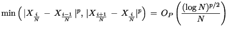
|
regardless of whether a (single) jump occurred or not over
![]() .
Since only finitely many terms differ,
.
Since only finitely many terms differ,
![$\displaystyle \sum_{j=1}^N\left[ \min \left(\vert X_{\frac{i}{N}}-X_{\frac{i-1}{N}}\vert^p, \vert X_{\frac{i+1}{N}}-X_{\frac{i}{N}}\vert^p\right) \, - \, \min \left(\vert Y_{\frac{i}{N}}-Y_{\frac{i-1}{N}}\vert^p, \vert Y_{\frac{i+1}{N}}-Y_{\frac{i}{N}}\vert^p\right) \right]\,$](img581.gif)
|
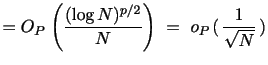
|
so neither consistency nor convergence in distribution is
affected by the presence of finite activity jumps. ![]()
A.7 Robust Neighborhood Truncation Estimators
We consider the
family of robust neighborhood truncation (RNT) estimators on a
block of ![]() i.i.d.
i.i.d.
![]() returns,
returns,
![]() . The estimator is
then constructed by taking the
. The estimator is
then constructed by taking the
![]() quantile of
quantile of ![]() unbiased estimators of
unbiased estimators of
![]() on the block. Denoting these
primitive estimators by
on the block. Denoting these
primitive estimators by
![]() , we
can write the RNT estimator as
, we
can write the RNT estimator as
![$\displaystyle RNT_N^{(j,\textbf{\emph{I}})}(p) \, = \, d_{(j,\textbf{\emph{I}})}(p) \, \frac{1}{(N-m+1)} \, \sum_{i=1}^{N-m+1} q_{j \,} \left[ \, \mathcal{E}_{1 \,}, \ldots , \, \mathcal{E}_{H \,} \right]$](img590.gif)
|
where the
![]() is a scaling
factor.
is a scaling
factor.
Lemma 9 Let
![]() be a positive even integer and assume that
the estimators
be a positive even integer and assume that
the estimators
![]() satisfy the conditions of Proposition 1 and Proposition 2, then the
robust neighborhood truncation estimator,
satisfy the conditions of Proposition 1 and Proposition 2, then the
robust neighborhood truncation estimator,
![]() , defined in
(35) is consistent
for
, defined in
(35) is consistent
for
![]() and satisfies a CLT.
and satisfies a CLT.
Proof. We need to verify the three
properties,(8)-(9) and
symmetry, of the ![]() function used in the
theorem are satisfied when
function used in the
theorem are satisfied when
![]() .
We deal with each condition in turn.
.
We deal with each condition in turn.
Clearly, if each primitive estimator
![]() is symmetric, so is
is symmetric, so is
![]() . Moreover,
if each
. Moreover,
if each
![]() satisfies a bound of the
type (8), so
will
satisfies a bound of the
type (8), so
will
![]() as it is
simply an order statistic of such bounded functionals. Finally,
assume that each
as it is
simply an order statistic of such bounded functionals. Finally,
assume that each
![]() satisfies (9). Except on
a null set, there exists a neighborhood around each m-tuple
satisfies (9). Except on
a null set, there exists a neighborhood around each m-tuple
![]() , on which
, on which
![]() for some
for some
![]() . Therefore it follows that also
. Therefore it follows that also
![]() satisfies
(9).
satisfies
(9).
![]()
Remark 10 Since the NT estimators (up to a scale factor) essentially are a special case of RNT, the lemma applies to these as well.
B Noise Robustness Properties of the
Ratio 
The ratio
![]() plays an important role for both
IV inference and jump attribution in finite samples. This section
extends the analysis of Huang and Tauchen (2005) to show that the
ratio
plays an important role for both
IV inference and jump attribution in finite samples. This section
extends the analysis of Huang and Tauchen (2005) to show that the
ratio ![]() has certain desirable robustness
features in the presence of microstructure noise. Following
Ait-Sahalia and Mykland (2005), we assume that the true price
process (
has certain desirable robustness
features in the presence of microstructure noise. Following
Ait-Sahalia and Mykland (2005), we assume that the true price
process (![]() ) is observed at
) is observed at ![]() discrete points in time with an independent stationary
(possibly autocorrelated) measurement error (
discrete points in time with an independent stationary
(possibly autocorrelated) measurement error (![]() ) that results in an MA error structure in observed
returns:
) that results in an MA error structure in observed
returns:
For simplicity, we focus the discussion here on the (RV,RQ) pairing and denote:
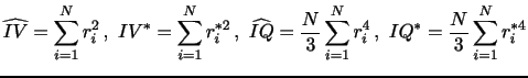
The presence of microstructure noise produces a bias in both the IQ and IV estimators of the form:
![$\displaystyle E[IQ^{*}]+\frac{N^{2}}{3}E[\varepsilon_{i}^{4}]+2NE[IV^{*}]E[\varepsilon_{i}^{2}]$](img619.gif)
|
|||
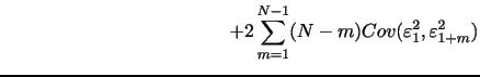
|
(35) |
In the special
case where
![]() is
serially uncorrelated and denoting the noise to signal ratio
is
serially uncorrelated and denoting the noise to signal ratio
![]() , the
expressions above simplify to,
, the
expressions above simplify to,
![$\displaystyle E[IV^{*2}] + 4E[IV^{*2}] (\lambda+\lambda ^2) + O\left(\frac{1}{N}\right)$](img631.gif)
|
(36) |
Under the null of
no jumps,
![]() are asymptotically
unbiased and consistent and,
are asymptotically
unbiased and consistent and,
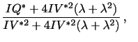 as
as |
The downward
bias of the limiting ratio depends on the noise-to-signal ratio
![]() and preaveraging of returns
therefore plays an important role in reducing
and preaveraging of returns
therefore plays an important role in reducing ![]() and the associated distortions.32 Moreover, for
sufficiently pre-averaged returns, there is very little evidence of
serial correlation, as pointed out by COP (2010), and the serially
uncorrelated noise case considered above is therefore the
empirically most relevant case.33In finite samples,
this downward bias is further compounded by a pure Jensen
(concavity) effect as readily seen from the Monte Carlo results for
the Brownian motion scenario Path by path, the Cauchy-Schwartz
inequality of course implies that
and the associated distortions.32 Moreover, for
sufficiently pre-averaged returns, there is very little evidence of
serial correlation, as pointed out by COP (2010), and the serially
uncorrelated noise case considered above is therefore the
empirically most relevant case.33In finite samples,
this downward bias is further compounded by a pure Jensen
(concavity) effect as readily seen from the Monte Carlo results for
the Brownian motion scenario Path by path, the Cauchy-Schwartz
inequality of course implies that
![]() must hold regardless of the noise structure or other
imperfections.
must hold regardless of the noise structure or other
imperfections.
In the presence
of other deviations from the Brownian null, forming the ratio
![]() may have a
stabilizing effect provided that the resulting distortion is
uniform and roughly proportional to squared returns since this will
lead to a cancelation in numerator and denominator. We see this
effect at work in the simulations with price discreteness but in
other instances, e.g., sparsity, it clearly fails. In cases
involving additive distortions such as jumps, there will be no
cancelation of biases and the ratio will tend to (in the case of
upward biases) diverge at high frequencies due to the scaling by N
in the numerator.
may have a
stabilizing effect provided that the resulting distortion is
uniform and roughly proportional to squared returns since this will
lead to a cancelation in numerator and denominator. We see this
effect at work in the simulations with price discreteness but in
other instances, e.g., sparsity, it clearly fails. In cases
involving additive distortions such as jumps, there will be no
cancelation of biases and the ratio will tend to (in the case of
upward biases) diverge at high frequencies due to the scaling by N
in the numerator.
C  and
and  estimators based
on pre-averaged returns
estimators based
on pre-averaged returns
Given
![]() equally-spaced (log) returns,
equally-spaced (log) returns,
![]() ,
,
![]() , we define corresponding
pre-averaged returns for any pre-averaging window size
, we define corresponding
pre-averaged returns for any pre-averaging window size ![]() :
:
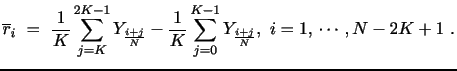
|
(37) |
An equivalent definition with analytically more tractable expression is given by:
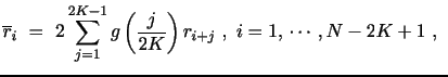
|
(38) |
where
![]() is the
pre-averaging kernel. We further define
is the
pre-averaging kernel. We further define
 as the finite sample analog of the variance scaling factor
![]() induced by
the pre-averaging kernel.34
induced by
the pre-averaging kernel.34
Consider the
following ![]() sub-samples of non-overlapping
pre-averaged returns:
sub-samples of non-overlapping
pre-averaged returns:
|
||
|
||
|
Let
![]() and
and
![]() ,
,
![]() denote the raw
denote the raw
![]() and
and ![]() estimates
obtained on each sub-sample of pre-averaged returns. Then the
pre-averaged (and sub-sampled) estimators
estimates
obtained on each sub-sample of pre-averaged returns. Then the
pre-averaged (and sub-sampled) estimators
![]() and
and
![]() for the full
set of pre-averaged returns
for the full
set of pre-averaged returns
![]() can
be defined as follows:
can
be defined as follows:
![$\displaystyle \frac{1}{2K} \sum_{i=1}^{2K} {\frac{1}{\psi}\widehat{IV}\left[\overline{S}_{i}\right]}$](img682.gif)
|
||
![$\displaystyle \frac{1}{2K} \sum_{i=1}^{2K} {\frac{1}{\psi^{2}}\widehat{IQ}\left[\overline {S}_{i}\right]}$](img685.gif)
|
After incorporating finite sample bias correction, these take the following final form that we use in our pre-averaged implementation of all estimators:
![$\displaystyle \widehat{IV}^{Adj}\left[ \overline{r}_{\cdot} \right]$](img686.gif)
|
![$\displaystyle \frac{1}{2K} \sum_{i=1}^{2K} {\frac{1}{\psi_{K}} \, \frac{\frac{N}{2K}} { \left \lfloor \frac{N-i+1}{2K} \right \rfloor } \widehat{IV} \left[\overline{S}_{i}\right]}$](img688.gif)
|
|
![$\displaystyle \widehat{IQ}^{Adj}\left[ \overline{r}_{\cdot} \right]$](img689.gif)
|
![$\displaystyle \frac{1}{2K} \sum_{i=1}^{2K} {\frac{1}{\psi_{K}^{2}} \, \frac{\left(\frac{N}{2K}\right)^ {2}}{ \left \lfloor \frac{N-i+1}{2K} \right \rfloor^{2}} \, \widehat{IQ}\left[\overline {S}_{i}\right]}$](img691.gif)
|
Consistency and asymptotic normality are clearly preserved by pre-averaging and sub-sampling, while noise-robustness improves. In particular, bounce-backs are near perfectly annihilated given that adjacent returns are subject to almost identical kernel weights. For further details on pre-averaging please refer to Podolskij and Vetter (2009) and Jacod, Li, Mykland, Podolskij and Vetter (2009) among others.
Footnotes
** Torben G. Andersen, Kellogg School of Management, Northwestern University, 2001 Sheridan Road, Evanston, IL 60208, USA; NBER; CREATES; [email protected].
Dobrislav Dobrev: Federal Reserve Board of Governors, 20th Street and Constitution Avenue NW, Washington, DC 20551, USA; [email protected].
Ernst Schaumburg: Federal Reserve Bank of New York, 33 Liberty Street, New York, NY 10045, USA; [email protected].
We are grateful to two anonymous referees as well as the editor, Jun Yu, for comments. We also thank participants at the 2010 SETA Conference at Singapore Management University and the "Nonlinear and Financial Econometrics Conference: A Tribute to A. Ronald Gallant," Toulouse, France, May 2011, the NBER-NSF Time Series Conference, Michigan State University, September 16-17, 2011, the 5th International Conference on Computational and Financial Econometrics, London, December 17-19, 2011, the 5th Annual SoFiE Conference - Oxford-Man Institute, June 20-22, 2012, the North American Summer Meeting of the Econometric Society, Evanston, June 28 - July 1, 2012, along with Federico Bandi, Peter R. Hansen, Andrew Patton, Peter C. B. Phillips and Kevin Sheppard for comments on an earlier draft. Excellent research assistance was provided by Patrick Mason.
Andersen gratefully acknowledges financial support from the NSF through a grant to the NBER and by CREATES funded by the Danish National Research Foundation.
The views in this paper are solely those of the authors and should not be interpreted as reflecting the views of the Board of Governors of the Federal Reserve System, the Federal Reserve Bank of New York or of any other person associated with the Federal Reserve System. Return to text
1. Corresponding measures were previously considered on an ad hoc basis, see, e.g., Schwert (1989), Hsieh (1991) and Zhou (1996). Return to text
2. Additional work regarding inference on the jump and continuous components of the return variation is developed in BNS (2004b, 2006), while general methodological insights were provided by Jacod and Protter (1998). Subsequently, market microstructure complications were addressed as part of the drive to exploit tick level data, see, e.g., Zhang, Mykland and Ait-Sahalia (2005), Bandi and Russell (2008), and Barndorff-Nielsen, Hansen, Lunde and Shephard, henceforth BNHLS, (2008). Return to text
3. Both studies explore the reliability of the procedures, but only under relatively ideal circumstances and not with a focus on the IQ estimator but rather the jump test statistic. Return to text
4. We rely on the MedRV/MedRQ estimators of Andersen, Dobrev and Schaumburg (2009) here, but any other sensible pair of robust IV and IQ estimators would suffice in this particular case as the evidence for a single significant jump is compelling and the associated empirical inference problem thus very straightforward. The robust estimators will be introduced later in the paper. Return to text
5. As a consequence, real-time predictions regarding the expected volatility over the following trading days will likely also be exaggerated on 2/26/2008 because the jump component of QV typically is much less persistent than the IV component, see, e.g., Andersen, Bollerslev and Diebold (2007). Return to text
6. Of course, the proofs for all our new results, provided in Appendix A, allow for a general drift term. Return to text
7. Naturally, additional dampening is
required to establish a CLT for the power variation measures. In
this case,
 for
for
![]() Return
to text
Return
to text
8. For IQ estimation based on a block
with five returns, we have
![]() . Hence, the largest normalization constant exceeds the smallest
one by a factor of several hundred; see Table 1 for additional
information. Return to text
. Hence, the largest normalization constant exceeds the smallest
one by a factor of several hundred; see Table 1 for additional
information. Return to text
9. For the integrated variance, these estimators may be interpreted as a redesigned version of the original Quantile Realized Variation, or QRV, estimator of Christensen, Oomen and Podolskij (COP) (2008), where it is applied to quantiles based on absolute rather than raw returns. The adaptation of QRV to cover the ADS (2012) nearest neighbor truncation estimators is discussed in COP (2010). This was also previously proposed during a conference discussion of COP (2010) by Kevin Sheppard, see also the comments in the realized_quantile_variance function in his Oxford MFE Toolbox. Return to text
10. In practice, finite sample complications can render the procedure less successful. One may want to avoid estimators that are highly sensitive to microstructure noise or jumps. Likewise, high correlation across estimators can generate optimal combinations that are extreme which may induce a degree of instability. Return to text
11. This is analogous to the use of linear combinations for the QRV estimator explored by COP (2008). Return to text
12. See, e.g., Jacod and Shiryaev (2003), Chapter IX, for an introduction to stable convergence. Return to text
13. We intend to apply these estimators in a setting with microstructure noise. As discussed in Section 4.2, this can be accommodated in the finite activity jump scenario via pre-averaging with a relatively large window size, resulting in a suboptimal convergence rate, but added robustness to noise. The literature on inference in the presence of infinite activity jumps and noise is limited. However, the findings for MPV estimators in Podolskij and Vetter (2009) and Hautsch and Podolskij (2010) suggest constructive results are feasible. Establishing formal results for this case falls outside the scope of the present paper. Return to text
14. In this notation, the initial "R"
references the RNT estimator, "Min" ("Med") signals that we
exploit the smallest (median) realization of the underlying NT
estimators, and "RQ" ("RV") indicates realized quarticity
(realized variance) estimation, that is ![]() (
(![]() ). It remains implicit that we take
). It remains implicit that we take
![]() , but retain only the three largest
absolute returns in constructing the estimator. Return to text
, but retain only the three largest
absolute returns in constructing the estimator. Return to text
15. P1: Retain only observations with time stamps between 9:30am and 4:00pm. P2: Retain only trades with positive prices. P3: Retain only trades originating from the main exchange (NYSE for all stocks except MSFT and INTL for which it is NASDAQ). T1: Delete entries with corrected trades. T2: Delete entries with abnormal sale condition. T3: If multiple trades occurred with the same time stamp, use the median price. T4: Delete entries with prices above the ask (or under the bid) by more than one bid-ask spread. Return to text
16. Analogous to the scaling factors
induced by the pre-averaging kernel, the efficiency with
subsampling depends on the pre-averaging scheme as well as the
length of the pre-averaging window relative to sample size. Hence,
applications involving subsampling must develop a suitable estimate
of the terms involving the efficiency factor ![]() in Section 3. One feasible
approach is simulation. Return to
text
in Section 3. One feasible
approach is simulation. Return to
text
17. Recognizing the downward bias, CPR develop an iterative rescaling procedure to alleviate this effect. Return to text
18. We confirm that our filtering
procedure under the BM null, applied to pre-averaged returns, is
active for about 1-in-![]() return blocks, while
the CPR filter is applied to roughly 1-in-
return blocks, while
the CPR filter is applied to roughly 1-in-![]() returns on average. Return to
text
returns on average. Return to
text
19. These return intervals span the range that is relevant for our empirical application. Findings based on a more comprehensive set of frequencies are reported in ADS (2011). Return to text
20. This choice facilitates effective cancelation of noise and outliers across the numerator and denominator. Return to text
21. Recall, we abandon the QRV style estimators for IQ due to the rapidly deteriorating performance in estimating higher order return variation under realistic market conditions. Return to text
22. The improved performance for TBQ is due to a fortuitous cancelation of the biases of the numerator and denominator under the BM null. Return to text
23. MPV and MPQ, in particular, as they are based on products of adjacent (absolute) returns. Return to text
24. When using tick sampled data, we are implicitly converting the calendar time scale to a tick scale, where time evolves linearly in tick time. This implies that the estimators are consistent for IQ in tick time, but not in calendar time. Importantly, in this setting the (tick time) IQ represents the relevant quantity for assessing the asymptotic variance of the (tick time based) IV estimator and for inference regarding jumps. Return to text
25. Ex post, we find no qualitative differences in results between the two samples, so we only report findings for the initial sample. The full set of results may be gleaned from ADS (2011). Return to text
26. Of course, this reflects the different philosophy behind the mild functional truncation filtering relative to TRQ and TBQ. The latter employ truncation of single returns as the primary tool for achieving jump robustness, and thus need to ensure that - asymptotically - all jumps are prevented from impacting the IQ estimator. This requires aggressive truncation and, inevitably, some truncation of diffusive returns, motivating the CPR adjustment to mitigate the resulting finite-sample bias, as discussed in Section 5. Return to text
27. We confirm that alternative robust volatility-of-volatility measures lead to qualitatively similar results. Return to text
28. The distance from the (non-functional filtered) RV curve to the set of robust IV measures provides an estimate of the average jump contribution to the quadratic return variation. Return to text
29. For each individual robust estimator, we regressed the difference of the daily realized power variation estimate across the distinct frequencies against the daily VoV measure, allowing for a separate intercept term but enforcing a common slope across the stocks. The detailed results are available in ADS (2011). Return to text
30. As argued in Barndorf-Nielsen,
Graversen, Podolskij, Jacod and Shephard (2006), henceforth BNGJPS,
this follows from working with the stopped versions of the
processes:
![]() and
and
![]() where
where
![]() and
and
![]() a.s. Return to text
a.s. Return to text
31. As for the volatility process, the specification may be generalized to infinite activity jump processes along the lines of Barndorff-Nielsen et al (2006c). Return to text
32. By Hölder's inequality,
![]() , so that the distortion due to
microstructure noise in general will result in a downward bias in
the limiting ratio. Return to
text
, so that the distortion due to
microstructure noise in general will result in a downward bias in
the limiting ratio. Return to
text
33. In the general case where
![]() is a MA(q) process:
is a MA(q) process:
![]() , we
have
, we
have
![$\displaystyle E[IV^{*2}] + E[IV^2] \left(\theta _1^2+\ldots+\theta _q^2+1\right){}^2 \lambda ^2+2 E[IV^2] \left(\theta _1^2+\ldots+\theta _q^2+1\right) \lambda+ O\left(\frac{1}{N}\right)$](img647.gif)
|
Return to text
34. Note that the factor 4 arises from the multiplication by 2 in equation (38). Return to text
This version is optimized for use by screen readers. Descriptions for all mathematical expressions are provided in LaTex format. A printable pdf version is available. Return to text