FEDS Notes
September 03, 2024
Convenience Yield as a Driver of r*
Balint Szoke, Ines Xavier and Francisco Vazquez-Grande1
The natural rate of interest, or $$r^*$$, corresponds to the short-term real interest rate that is consistent with full employment and price stability, after all temporary shocks have abated. The most popular framework to estimate $$r^*$$ is Laubach and Williams (2003) and Holston, Laubach, and Williams (2017, 2023) (henceforth HLW). Their framework defines $$r^*$$ as the sum of two unobservable components, $$$$r^*_t = g_t + z_t, \ (1)$$$$ where $$g$$ denotes the trend growth rate of potential output, and $$z$$ captures other time- varying drivers of the natural rate that are not explicitly modeled. HLW estimates that $$z$$ accounts for most to the decline in $$r^*$$ since the late 2000s. Because $$z$$ is modelled as a residual component of $$r^*$$, the economic forces behind the decline in the natural rate since the 2000s remain unknown.
In this note, we present statistical evidence that over the past two decades, the decline of $$z$$ in HLW's framework is largely explained by the increases in convenience yield of U.S. Treasury securities. To show this, we generalize the model of HLW by introducing a wedge between the interest rate of privately issued securities—which influences private sector saving and investment decisions—and the yield of government issued safe assets. This wedge is usually referred to as the convenience yield of Treasury securities and is driven by the supply and demand for liquid and safe assets, government debt net issuance, financial sector regulation, as well as changes in foreign and domestic demand for U.S. debt.
Intuitively, changes in the convenience yield affect the estimation of $$r^*$$ through forces that may lead to a reallocation of real resources in the economy. For example, shocks that (persistently) increase the relative demand for safe and liquid assets tend to shift savings away from private assets and toward government securities, reducing private investment and therefore putting downward pressure on $$r^*$$.2
Our model's estimates suggest that over the past five decades changes in the natural rate of interest are accounted for by both changes in the growth rate of potential output and in the trend convenience yield of government securities. Since the Global Financial Crisis (GFC), however, our estimates suggest that changes in the convenience yield explain most of the $$r^*$$ dynamics. We also find that accounting for the wedge between private borrowing costs and safe and liquid interest rates improves the inference of $$r^*$$, in the sense that the uncertainty around the estimates of $$r^*$$ is significantly smaller relative to what is typically reported in the literature.
In the first quarter of 2024, we estimate that $$r^*$$ is about 75 basis points with a 68% confidence band ranging approximately between of 50 and 100 basis points, and that the stance of monetary policy is significantly restrictive, at about the same level that prevailed before the 2001 and 2008 recessions.
Related literature. In the macro-banking literature, the distinction between public and private borrowing costs is at the core of the transmission of monetary policy through the financial intermediary sector (Goodfriend and McCallum, 2007; Piazzesi et al., 2022). In this literature, the policy rate directly affects the yields on short-term government securities, but the pass-through on private rates is imperfect because government securities carry a premium—the convenience yield—relative to other private sector assets. As yields of private assets ultimately influence consumption and investment decisions, changes in the convenience yield affect the transmission of monetary policy to private saving and investment decisions.
The economic literature has provided some support for a relationship between $$r^*$$ and slow-moving economic developments that persistently affect aggregate demand and supply, such as trend GDP growth, demographic change, trends in income inequality, capital market integration, and the level of government debt.3 Our work is closely related to Del Negro et al. (2017), who use a reduced-form estimation approach and a DSGE model to empirically assess the importance of movements in the convenience yield for estimating $$r^*$$. In contrast, we estimate $$r^*$$ within a stylized macroeconomic-model—featuring both an IS equation and a forward-looking Phillips curve—that identifies $$r^*$$ as the level of the real rate that keeps inflation at target and output at potential and that is flexible enough to fit the time series dynamics of output, inflation, corporate yields, the policy rate and long-term corporate and Treasury yields.
Chikis et al. (2023) study the drivers of $$r^*$$ through the lens of an endogenous growth model that, like our macroeconomic model, allows for a wedge between the risk-free rate and the private return on investment. They find that a persistent increase in the required excess return on investment over the risk-free rate at the time of the GFC—consistent with the increase in the convenience yield that we estimate during this period—can reduce innovation, depress risk free rates, and explain both a decrease in the growth rate of aggregate productivity and of $$r^*$$ since the GFC.
Economic and Statistical Framework
We incorporate the convenience yield into a stylized macroeconometric model de- scribing the output gap and inflation dynamics. We build on the work of HLW and Del Negro et al. (2017) and use Bayesian techniques to estimate the permanent component of output, inflation, convenience yield, real rates, and the natural interest rate. Szoke, Vazquez-Grande, and Xavier (2024) provides further technical details on the econometric model and the estimation procedure used in this note.
Our economic framework is motivated by the observation that government issued safe-assets are traded at a premium—due to their safety and liquidity properties—relative to private sector securities even after accounting for risk-premia. That is, the real risk-free rate faced by the private sector—a rate that is relevant for output and inflation—does not move one-to-one with the real rate of Treasury securities.
We define the natural real rate faced by the private sector $$\left({\overline{r}}^{ps}\right)$$ as the default free real interest rate that would prevail after all transitory disturbances have abated. Following HLW we assume that this rate is determined by the sum of two unobservable components: trend output growth (g) and a residual term (z) that capture the forces that drive equilibrium real rates beyond trend growth: $$$$\bar{r}^{ps}_t := g_t + z_t. \ (2)$$$$
Similar to HLW, we specify a simple aggregate demand and aggregate supply model to characterize the dynamic of the output gap ($$\widetilde{y}$$) and the deviations of inflation from target ($$\widetilde{\pi}$$). In our model, the level of the output gap and the deviations of inflation from target are ultimately affected by the deviations of the one-period real risk-free rate faced by the private sector ($$r^{ps}$$) and the natural rate $$\left({\overline{r}}^{ps}\right)$$:
$$$$\tilde{y}_t = a_1 \tilde{y}_{t-1} + a_2 \tilde{y}_{t-2} + \frac{a_r}{2}(\tilde{r}^{ps}_{t} + \tilde{r}^{ps}_{t-1}) + \sigma_1 \varepsilon_{1, t} \ (3)$$$$ $$$$\tilde{\pi}_t = b_{\pi} E_t[\tilde{\pi}_{t+1}] + b_Y \tilde{y}_{t-1} + \sigma_2 \varepsilon_{2, t} \ (4)$$$$ where $${\widetilde{r}}_t^{ps}$$ is the real rate gap faced by the private sector $${\widetilde{r}}_t^{ps}≔rtps-rtps$$, and $$E_t\left[{\widetilde{\pi}}_{t+1}\right]$$ is one period ahead inflation expectations.4
Relative to HLW, in our setting the convenience yield ($$cy$$), is the spread between the real risk-free rate faced by the private sector ($$r^{ps}$$) and the rate of government issued securities ($$r$$) $$$$cy_t := r^{ps}_t - r_t \ (5)$$$$ and $$\bar{cy}$$ denotes the level of the convenience yield once all transitory shocks have dissipated.
Using definitions (2) and (5) we can rewrite the private sector real rate gap in terms of the real policy rate gap
$$$$\tilde{r}^{ps}_{t} = (r^{ps}_{t} - \bar{r}^{ps}_{t}) = (r_t + cy_t - (g_t + z_t)) = (r_t - (g_t + z_t - \overline{cy}_t)) + (cy_t - \overline{cy}_t) \ (6)$$$$
leading us to our definition of the natural policy rate
$$$$r^*_t := g_t + z_t - \overline{cy}_t. \ (7)$$$$
Notice that relative to HLW's definition in equation (1), changes in the (trend of) convenience yield directly affect the level of the natural rate.
To estimate the model, we use quarterly data between 1962 and 2024 on real GDP, core PCE inflation, the nominal effective federal funds rate, and the convenience yield. Following Krishnamurthy and Vissing-Jorgensen (2012), we measure the convenience yield of Treasury securities as the spread between Aaa corporate bond yields and the yield on the 10-year Treasury bond.5,6 This measure is plotted in Figure 1. As shown, the convenience yield presents an upward trend that extends from the early 80s to the early 2000's, increasing by about 1 percentage point, on net, over the period. Between the early-2000's and the GFC, as the securitization of private debt boomed, the convenience yield declined significantly, only to jump up in the flight to safety episode at the onset of the GFC. The convenience yield remained elevated in the recovery post GFC and started a downward trend in the mid-2010's, temporarily interrupted by the Covid recession.
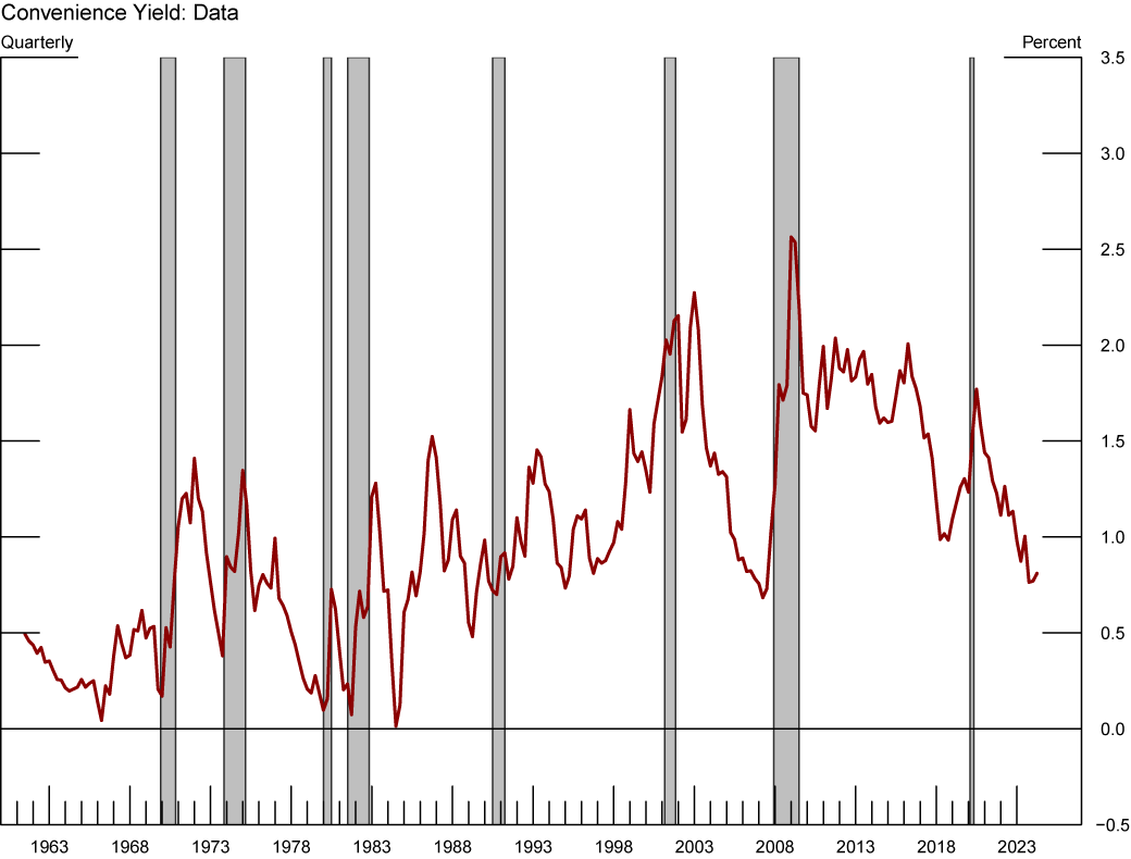
Note: The figure above shows difference in yields of safe (Aaa) corporate bonds and the 10-year Treasury yield in percent yield. Grey-shaded areas denote periods of recession as denoted by the National Bureau of Economic Research: December 1969-November 1970, November 1973-March 1975, January 1980-July 1980, July 1981-November 1982, July 1990-March 1991, March 2001-November 2001, December 2007-June 2009, February 2020-April 2020.
Source: Staff’s calculations.
Convenience Yield measured as the spread between the yield on safe (Aaa) corporate bonds and the 10-year Treasury yield. Gray shaded bars denote periods of recession as dated by the National Bureau of Economic Research: December 1969-November 1970, November 1973-March 1975, January 1980-July 1980, July 1981-November 1982, July 1990-March 1991, March 2001-November 2001, December 2007-June 2009, and February 2020-April 2020.
Results
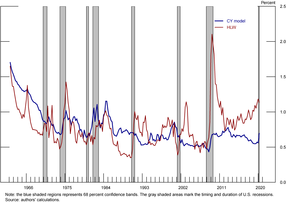
The solid blue line in Figure 2 plots our median estimate of $$r^*$$, with the blue shaded area representing a 68% confidence set. For comparison, the solid red line depicts the estimated $$r^*$$ from the latest version of the model available at the Federal Reserve Bank of New York (FRBNY) website. Although both estimates of $$r^*$$ generally exhibit a downward trend throughout the sample and are on average close to each other, the drivers behind this trend come from different sources which explain some of the temporary differences between the two measures.
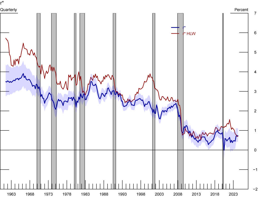
Note: The figure above shows our $$r^*$$ estimates and 68% confidence bands compared with the $$r^*$$ estimates of Holston, Laubach, and Williams (2017, 2023). Grey-shaded areas denote periods of recession as denoted by the National Bureau of Economic Research: December 1969-November 1970, November 1973-March 1975, January 1980-July 1980, July 1981-November 1982, July 1990-March 1991, March 2001-November 2001, December 2007-June 2009, February 2020-April 2020.
Sources: Federal Reserve Bank of New York, staff’s calculations.
Median estimate of $$r^*$$ under our baseline specification (blue) and the estimation of HLW (red) from FRBNY. The shaded blue area represents 68% confidence bands for our estimate. Gray shaded bars denote periods of recession as dated by the National Bureau of Economic Research: December 1969-November 1970, November 1973-March 1975, January 1980-July 1980, July 1981-November 1982, July 1990-March 1991, March 2001-November 2001, December 2007-June 2009, and February 2020-April 2020.
Figure 3 plots our estimates of $$r^*$$ and its three components as described in equation (7).7 Like HLW, we find that the growth rate of potential output, $$g$$, has trended downward, on net, since 1962, as depicted by the solid black line.8 However, we also find that another important driver of the decline in $$r^*$$ is the trend in the convenience yield (the solid green line). From the early 80s to the mid-2010s, we estimate that $$r^*$$ declined 2.25 percentage points, on net, with the increase in the convenience yield accounting for about 60 percent of the net decline in $$r^*$$ over this period, and the rest explained by the decline in trend growth.
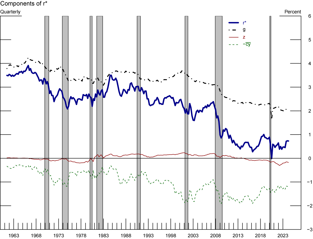
Note: The figure shows $$r^*$$ and its components. Grey-shaded areas denote periods of recession as denoted by the National Bureau of Economic Research: December 1969-November 1970, November 1973-March 1975, January 1980-July 1980, July 1981-November 1982, July 1990-March 1991, March 2001-November 2001, December 2007-June 2009, February 2020-April 2020.
Sources: Staff’s calculations.
Median estimates of $$r^*$$ and its components: $$r^\ast=g+z-\bar{cy}$$. Gray shaded bars denote periods of recession as dated by the National Bureau of Economic Research: December 1969-November 1970, November 1973-March 1975, January 1980-July 1980, July 1981-November 1982, July 1990-March 1991, March 2001-November 2001, December 2007-June 2009, and February 2020-April 2020.
Our estimate of the trend in the convenience yield is consistent with key U.S. macroeconomic and financial developments over the past five decades. For example, in the 70s and until the early 80s, the trend in convenience yield declined, on net, reflecting a period of high and persistent inflation, and rebounded in the mid-80s, as inflation and inflation expectations began to moderate. High inflation and inflation risk, deteriorate the "moneyness" property of government issued long-maturity securities (prompting substitution for other money-like assets), decreasing their convenience yield.9 Since the mid-2000s, we estimate that the trend in convenience yield declined notably, consistent with the US securitization boom (Mian and Sufi, 2009) that contributed to increase the collateral value of private sector safe debt, lowering the yields of privately issued safe assets relative to those of Treasury securities, and reducing the convenience yield.10 Also, the normalization of the Federal Reserve balance sheet starting in 2017, that increased the Treasury securities available to the public, coincides with a decrease in the trend of convenience yield.
The convenience yield also helps explain why our estimates of $$r^*$$ remained subdued in the years post GFC. In 2008 the brisk increase in trend convenience yield coincides with the expansion of the Federal Reserve balance sheet, and the adoption of leverage regulation and enhanced prudential standards for large banks that strengthened the requirement for holding high-quality liquid assets. The large increase in convenience yield post GFC together with a modest decrease in trend growth drive our estimates of low $$r^*$$ during this period. Our findings are consistent with the estimates of $$r^*$$ in HLW, with the important difference that while they assign the decline in $$r^*$$ post-GFC to the notable fall their exogenous factor $$z$$ (see figure 4), we identify such decline in $$r^*$$ to the steep rise in the (trend) convenience yield.
Turning to our estimate of the (residual) component $$z$$, depicted by the solid red line in figure 3, we find that, after accounting for the convenience yield on U.S. Treasury yields, this latent variable loses much of its explanatory power of the secular decline in $$r^*$$. Figure 4 makes this point more explicitly by plotting the estimated path of the latent $$z$$ under our specification (the blue line) and the estimated $$z$$ of HLW. While the decline in $$z$$ contributes significantly to the downward trend in HLW's estimate of $$r^*$$ since the early 1990s, our estimate of $$z$$ is not statistically different from zero and varies little throughout the sample. This result suggests that the trend in convenience yield offers an economic interpretation of the non-growth component of $$r^*$$ identified in HLW.
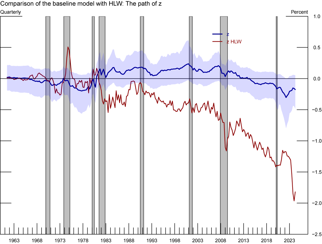
Note: The figure above shows our $$z$$ estimates and 68% confidence bands compared with the $$z$$ estimates of Holston, Laubach, and Williams (2017, 2023). Grey-shaded areas denote periods of recession as denoted by the National Bureau of Economic Research: December 1969-November 1970, November 1973-March 1975, January 1980-July 1980, July 1981-November 1982, July 1990-March 1991, March 2001-November 2001, December 2007-June 2009, February 2020-April 2020.
Sources: Federal Reserve Bank of New York, staff’s calculations.
Median estimate of the $$z$$ process under two models: our baseline specification (blue) and the estimation of HLW (red) form the FRBNY. The shaded area represents the 68 percent confidence band for our estimate of $$z$$. Gray shaded bars denote periods of recession as dated by the National Bureau of Economic Research: December 1969-November 1970, November 1973-March 1975, January 1980-July 1980, July 1981-November 1982, July 1990-March 1991, March 2001-November 2001, December 2007-June 2009, and February 2020-April 2020.
Another important finding of our approach is that incorporating data on the convenience yield leads to more precise estimates of $$r^*$$ relative to other models in the literature. After 2000, the size of the confidence bands is notably smaller than those from the HLW model. This is shown in figure 5, which plots the width of 68% confidence bands for our estimate of $$r^*$$ and for that of HLW, with higher values representing higher uncertainty.11 At each point in time, the vertical distance between the two lines in figure 5, represents the difference in precision between the two models. The increase in precision is noticeable in the latest part of our sample, when the convenience yield becomes more informative for the path of $$r^*$$. The higher precision suggests that the signal provided by the spread between government and corporate safe assets is informative for the estimation of $$r^*$$. In particular, since the GFC, the width of our 68% confidence bands is about 50% lower, on average, than that of HLW.
Note: The figure above shows the width of our 68% confidence bands of $$r^*$$ compared with those of Holston, Laubach, and Williams (2017, 2023). Grey-shaded areas denote periods of recession as denoted by the National Bureau of Economic Research: December 1969-November 1970, November 1973-March 1975, January 1980-July 1980, July 1981-November 1982, July 1990-March 1991, March 2001-November 2001, December 2007-June 2009, February 2020-April 2020.
Sources: Federal Reserve Bank of New York, staff’s calculations.
Estimates of the size of the 68% $$r^*$$ confidence bands under two models, our model specification (blue) and the specification of HLW (2017) (red). Gray shaded bars denote periods of recession as dated by the National Bureau of Economic Research: December 1969-November 1970, November 1973-March 1975, January 1980-July 1980, July 1981-November 1982, July 1990-March 1991, March 2001-November 2001, December 2007-June 2009, and February 2020-April 2020.
Finally, Appendix B compares our estimate of the output gap with that of HLW and the Congressional Budget Office. We take the improvement in the measurement of the cyclical dynamics of U.S. output over HLW as further evidence that the inclusion of the convenience yield in the estimation of $$r^*$$ provides a valuable signal to the model.
The Stance of Policy in the Current Tightening Cycle
Figure 6 plots our model's estimate of the monetary policy stance ($$r-r^*$$), defined as the gap between the ex-ante real rate, $$r$$,—i.e., the observed policy rate netted of the model-consistent one-quarter ahead (annualized) inflation expectations—and the measure of $$r^*$$. Focusing on the years after the Covid recession, we estimate that the monetary response to the Covid pandemic created a negative real policy rate gap, as the policy stance eased notably in mid-2020. In contrast, during the current monetary policy tightening cycle, beginning in early 2022, the stance of policy tightened at an unprecedented speed. According to our estimates policy moved to contractionary territory in mid-2023 and continued to tighten over the second half of the year. We estimate the policy stance in 2024Q1 to be restrictive with the real rate about 1.15 percentage points above the natural rate, at about the same level that prevailed before the 2001 and 2008 recessions.12
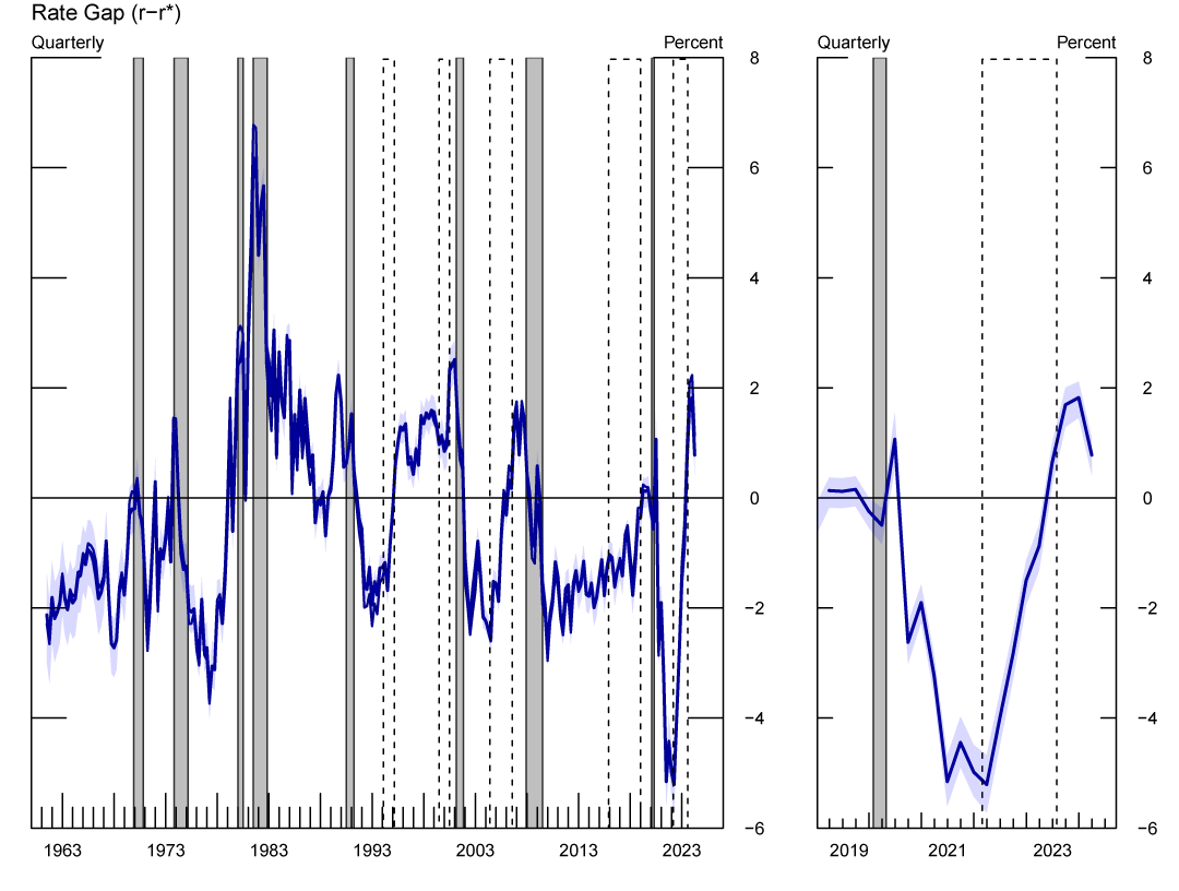
Note: The figures show the stance of Policy ($$r-r^*$$). Positive (negative) values denote real rates above (below) the natural rate of interest. Grey-shaded areas denote periods of recession as denoted by the National Bureau of Economic Research: December 1969-November 1970, November 1973-March 1975, January 1980-July 1980, July 1981-November 1982, July 1990-March 1991, March 2001-November 2001, December 2007-June 2009, February 2020-April 2020. The dashed bars represent monetary policy tightening cycles: February 1994-March 1995, July 1999-July 2000, June 2004-August 2006, December 2015-July 2018, and March 2022-present.
Source: Staff’s calculations.
The stance of policy or the real policy rate gap is defined as the difference between the ex-ante real policy rate and $$r^*$$. The ex-ante real policy rate is computed by subtracting the model's estimate of inflation expectations over the upcoming three months (annualized) from the policy rate. The shaded blue areas represent 68% confidence bands. Gray shaded bars denote periods of recession as dated by the National Bureau of Economic Research: December 1969-November 1970, November 1973-March 1975, January 1980-July 1980, July 1981-November 1982, July 1990-March 1991, March 2001-November 2001, December 2007-June 2009, and February 2020-April 2020. The dashed bars represent monetary policy tightening cycles: February 1994-March 1995, July 1999-July 2000, June 2004-August 2006, December 2015-July 2018, March 2022-present. Tightening cycles are defined to start on the month of the first federal funds rate increase and end after the last rate hike.
References
Acharya, V. V. and T. Laarits (2023, November). "When do Treasuries Earn the Convenience Yield? — A Hedging Perspective". NBER Working Papers 31863, National Bureau of Economic Research, Inc.
Bernanke, B. S. (2005). "The global saving glut and the U.S. current account deficit".
Technical report, Homer Jones Lecture, Federal Reserve Bank of St. Louis.
Chikis, C. A., J. Goldberg, and D. Lopez-Salido (2023). "Financial discounts and creative-destruction dynamics". Technical report, Board of Governors of the Federal Reserve System (U.S.).
Del Negro, M., D. Giannone, M. P. Giannoni, and A. Tambalotti (2017). "Safety, liquidity, and the natural rate of interest". Brookings Papers on Economic Activity 2017 (1), 235–316.
Ferreira, T. R. T. and S. Shousha (2021, April). "Supply of Sovereign Safe Assets and Global Interest Rates". International Finance Discussion Papers 1315, Board of Governors of the Federal Reserve System (U.S.).
Gagnon, E., B. K. Johannsen, and D. Lopez-Salido (2021, June). "Understanding the New Normal: The Role of Demographics". IMF Economic Review 69 (2), 357–390.
Goodfriend, M. and B. T. McCallum (2007). "Banking and interest rates in monetary policy analysis: A quantitative exploration". Journal of Monetary Economics 54 (5), 1480–1507.
Gust, C. J. and A. Skaperdas (2024, May). "Government Debt, Limited Foresight, and Longer-term Interest Rates". Finance and Economics Discussion Series 2024-027, Board of Governors of the Federal Reserve System (U.S.).
Holston, K., T. Laubach, and J. C. Williams (2017). "Measuring the natural rate of interest: International trends and determinants". Journal of International Economics 108, S59 – S75. 39th Annual NBER International Seminar on Macroeconomics.
Holston, K., T. Laubach, and J. C. Williams (2023, June). "Measuring the Natural Rate of Interest after COVID-19". Working Paper Series 1063, Federal Reserve Bank of New York Staff Reports.
Krishnamurthy, A. and A. Vissing-Jorgensen (2012). "The aggregate demand for Treasury debt". Journal of Political Economy 120 (2), 233–267.
Laubach, T. and J. C. Williams (2003). "Measuring the natural rate of interest". Review of Economics and Statistics 85 (4), 1063–1070.
Lunsford, K. G. and K. D. West (2019, October). "Some Evidence on Secular Drivers of US Safe Real Rates". American Economic Journal: Macroeconomics 11 (4), 113– 139.
Mian, A., L. Straub, and A. Sufi (2021, September). "What explains the decline in $$r^*$$? Rising income inequality versus demographic shifts". Working Papers 2021-12, Princeton University. Economics Department.
Mian, A. and A. Sufi (2009, 11). "The Consequences of Mortgage Credit Expansion: Evidence from the U.S. Mortgage Default Crisis". The Quarterly Journal of Economics 124 (4), 1449–1496.
Piazzesi, M., C. Rogers, and M. Schneider (2022). "Money and banking in a new Keynesian model".
Platzer, J. and M. Peruffo (2022, February). "Secular Drivers of the Natural Rate of Interest in the United States: A Quantitative Evaluation". IMF Working Papers 2022/030, International Monetary Fund.
Szoke, B., F. Vazquez-Grande, and I. Xavier (2024). "The drivers of $$r^*$$: Accounting for Treasuries' convenience yield". Working Paper.
Waller, C. J. (2024, May 24). "Some thoughts on $$r^*$$: Why did it fall and will it rise?" Speech at the Reykjavik Economic Conference, Reykjavik, Iceland.
Appendix
A. Measuring the Convenience Yield
In this section, we discuss the properties of our preferred measure of the convenience yield and consider an alternative gauge.
Our benchmark measure of the convenience yield is equal to the spread between Moody's seasoned Aaa corporate bond yields and long-term US Treasury bonds of comparable maturities, following Krishnamurthy and Vissing-Jorgensen (2012). As a set of securities that virtually never default, Aaa corporate bonds carry approximately the same safety premium as Treasuries. However, they are less liquid, so they enjoy less of a liquidity premium compared to Treasuries. As a result, we interpret our benchmark measure of the convenience yield as primarily capturing the liquidity premium attached to U.S. Government securities.
An alternative measure of the wedge between the policy rate and private borrowing costs is the spread between Baa corporate bonds and Treasuries, as also discussed in Krishnamurthy and Vissing-Jorgensen (2012). Since Baa corporate bonds are less safe and less liquid than Treasuries, this spread captures both safety and liquidity premia. As a robustness check, and to allow for the possibility that longer-run trends in safety premia might also affect the level of $$r^*$$, we re-estimate our model with the convenience yield being approximated by the Baa spread (instead of the Aaa spread). The blue line in figure 7 shows the path of the posterior median estimate of $$r^*$$ from this alternative specification with the blue band representing the corresponding 68% confidence set. For comparison, the red solid line depicts the estimated $$r^*$$ from the benchmark model. Although using the Baa corporate bonds spread leads, on average, to slightly lower estimates of $$r^*$$, this difference is not statistically significant, and thus the results highlighted in the previous section remain valid.
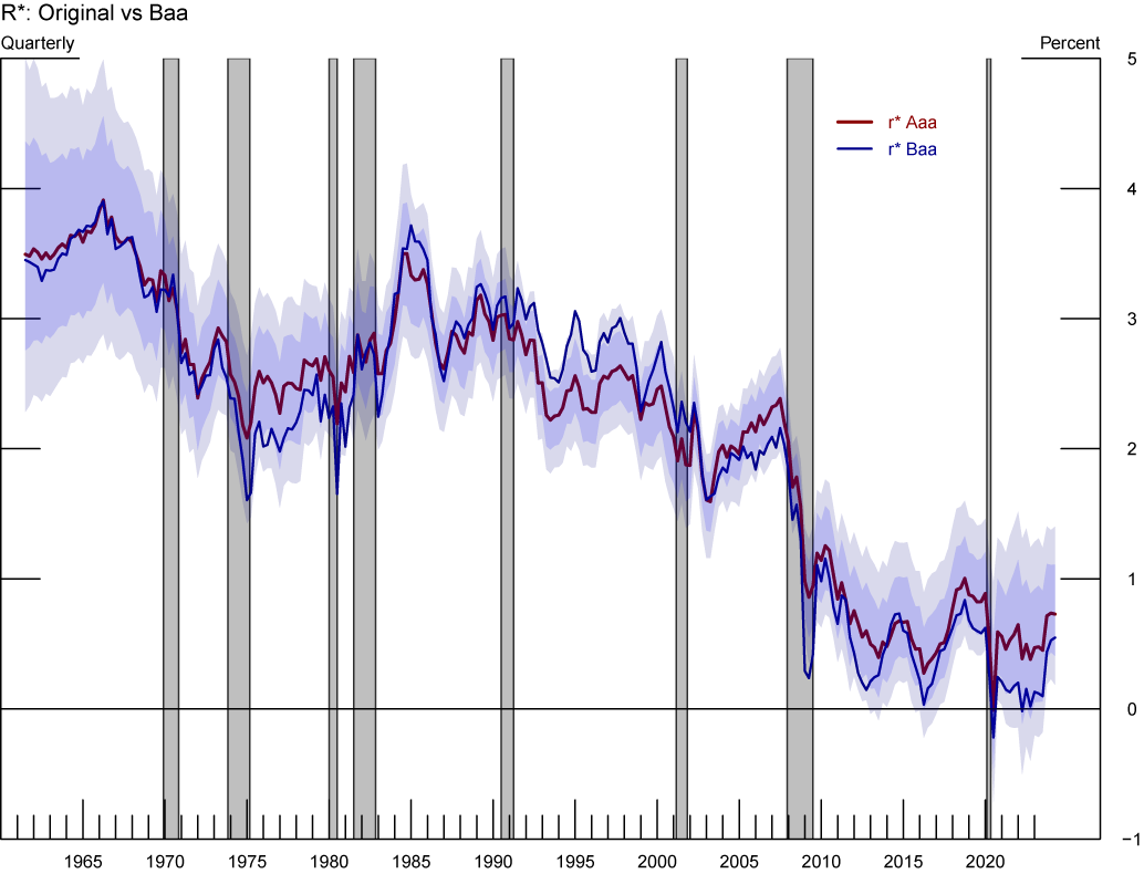
Note: The figure shows estimates of $$r^*$$ based on Different series of US Corporate Yields. Grey-shaded areas denote periods of recession as denoted by the National Bureau of Economic Research: December 1969-November 1970, November 1973-March 1975, January 1980-July 1980, July 1981-November 1982, July 1990-March 1991, March 2001-November 2001, December 2007-June 2009, February 2020-April 2020.
Source: Staff’s calculations.
The blue and light-grey shaded regions represent the 68 and 95 percent confidence bands, respectively, for the estimate of $$r^*$$ computed using Aaa corporate yields. Gray shaded bars denote periods of recession as dated by the National Bureau of Economic Research: December 1969-November 1970, November 1973-March 1975, January 1980-July 1980, July 1981-November 1982, July 1990-March 1991, March 2001-November 2001, December 2007-June 2009, and February 2020-April 2020.
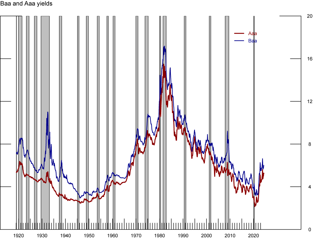
Taking a closer look at the path of Moody's seasoned Baa and Aaa corporate bond yields further helps understand the previous result. As shown in figure 8, the time-series of both corporate bond yields positively correlates over the past 100 years. In particular, the long-run trends of both series co-move throughout our sample with a transitory difference that reflects the time-varying risk-premium present in riskier corporate bonds. After conducting econometric tests, we find that the two series are cointegrated with cointegrating vector (1, −1), which in turn implies that the risk-premium commanded by Baa bonds relative to Aaa bonds is stationary (and, thus, does not significantly alter the estimate of the trend convenience yield relevant for our measure of $$r^*$$).

Note: The figure shows US Corporate Yields. Grey-shaded areas denote periods of recession as dated by the National Bureau of Economic Research: August 1918-March 1919, January 1920-July 1921, May 1923-June 1924, October 1926-November 1927, August 1929-March 1933, May 1937-June1938, February 1945-October 1945, November 1948-October 1949, July 1953-May 1954, August 1957-April 1958, April 1960-February 1961, December 1969-November 1970, November 1973-March 1975, January 1980-July 1980, July 1981-November 1982, July 1990-March 1991, March 2001-November 2001, December 2007-June 2009, February 2020-April 2020.
Sources: Moody’s
Gray shaded bars denote periods of recession as dated by the National Bureau of Economic Research: December 1969-November 1970, November 1973-March 1975, January 1980-July 1980, July 1981-November 1982, July 1990-March 1991, March 2001-November 2001, December 2007-June 2009, and February 2020-April 2020.
We choose the spread between Aaa corporate bond yields and US Treasury bonds as our benchmark measure of the convenience yield for three reasons. First, we think this spread provides a closer proxy for the convenience yield defined in the theoretical literature as it not confounded by risk premia. Second, as previously discussed, the results do not strongly depend on which measure of the convenience yield is used. This is unsurprising as the two spreads have similar trends, as can be seen in figure 9. Finally, we find that the Baa corporate bonds spread is more volatile than the Aaa corporate bonds spread and, therefore, our filtering of the convenience yield becomes somewhat less informative for the estimation of $$r^*$$ within our framework (as the algorithm has a harder time separating the transitory volatile component that correspond to risk premia and the permanent component that comes from convenience yield).
Note: The figure shows the Convenience Yield trend using different bond spreads (Aaa vs Baa). Grey-shaded areas denote periods of recession as denoted by the National Bureau of Economic Research: December 1969-November 1970, November 1973-March 1975, January 1980-July 1980, July 1981-November 1982, July 1990-March 1991, March 2001-November 2001, December 2007-June 2009, February 2020-April 2020.
Source: Staff’s calculations.
Gray shaded bars denote periods of recession as dated by the National Bureau of Economic Research: December 1969-November 1970, November 1973-March 1975, January 1980-July 1980, July 1981-November 1982, July 1990-March 1991, March 2001-November 2001, December 2007-June 2009, and February 2020-April 2020.
B. Estimates of the Output Gap
Figure 10 compares our estimated output gap with those resulting from the estimation of HLW and the Congressional Budget Office (CBO). As shown, our model captures the cyclical dynamic of U.S. output well. Importantly, our output gap estimate is stationary throughout the sample, trending up during expansions, peaking at the onset of recessions and bottoming at the beginning of recoveries. Its range of variation is lower than that of the other metrics displayed in figure 10. This is likely driven by our estimates of trend growth $$g$$, which is less volatile and less cyclical than in HLW.
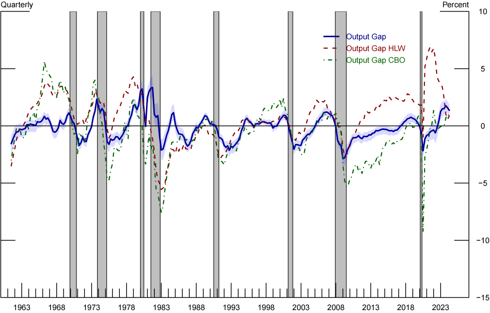
Note: The figure shows our estimated output gap compared with that of Holston, Laubach, and Williams (2017, 2023), and the Congressional Budget Office (CBO). Grey-shaded areas denote periods of recession as denoted by the National Bureau of Economic Research: December 1969-November 1970, November 1973-March 1975, January 1980-July 1980, July 1981-November 1982, July 1990-March 1991, March 2001-November 2001, December 2007-June 2009, February 2020-April 2020.
Sources: Federal Reserve Bank of New York, Congressional Budget Office, staff’s calculations.
Three estimates of the output gap, the one from our baseline specification that accounts for the convenience-yield of Treasuries (blue), the estimate of HLW (red) and the estimate of the CBO (green). The grey shaded regions mark the time of NBER- dated recessions.
From the mid-80s to the GFC, all three measures of the estimated output gap track each other closely. However, after the GFC, the estimates from the HLW model recover much faster than our estimates or that of the CBO. Our measure of the output gap remains negative until 2017. After the Covid recession, our estimate also recovers more slowly than that of HLW and, in contrast with that of the CBO, our gap became positive in 2022 and continued to widen since then. We take the improvement in the measurement of the cyclical dynamics of U.S. output over HLW as further evidence that the inclusion of the convenience yield in the estimation of $$r^*$$ provides a valuable signal to the model. In particular, the size of the 68% confidence bands is reduced by about 50%, on average, since the Great Financial Crisis with respect to those of HLW.
C. Additional Figures
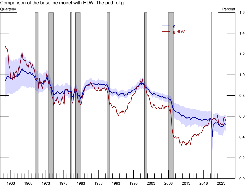
Note: The figure shows our estimated $$g$$ compared with that of Holston, Laubach, and Williams (2017, 2023). Grey-shaded areas denote periods of recession as denoted by the National Bureau of Economic Research: December 1969-November 1970, November 1973-March 1975, January 1980-July 1980, July 1981-November 1982, July 1990-March 1991, March 2001-November 2001, December 2007-June 2009, February 2020-April 2020.
Sources: Federal Reserve Bank of New York, staff’s calculations.
Two estimates of trend growth, the one from our baseline specification that accounts for the convenience-yield of Treasuries (blue) and the estimate of HLW provided by FRBNY (red). Gray shaded bars denote periods of recession as dated by the National Bureau of Economic Research: December 1969-November 1970, November 1973-March 1975, January 1980-July 1980, July 1981-November 1982, July 1990-March 1991, March 2001-November 2001, December 2007-June 2009, and February 2020-April 2020. The units are quarterly (not annualized).
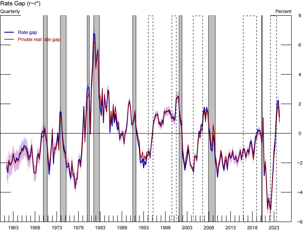
Note: The figure Real Policy and Private Sector Rate Gaps. Grey-shaded areas denote periods of recession as denoted by the National Bureau of Economic Research: December 1969-November 1970, November 1973-March 1975, January 1980-July 1980, July 1981-November 1982, July 1990-March 1991, March 2001-November 2001, December 2007-June 2009, February 2020-April 2020.
Source: Staff’s calculations.
The real policy rate gap is defined as the difference between the ex-ante real policy rate and $$r^\ast≔g+z-cy$$ and is plotted in blue. The private sector real rate gap is defined as the difference between the ex-ante one-period real private sector rate and $${\bar{r}}^{ps}≔g+z$$ and is plotted in red. The shaded blue areas represent 68\% confidence bands. Gray shaded bars denote periods of recession as dated by the National Bureau of Economic Research: December 1969-November 1970, November 1973-March 1975, January 1980-July 1980, July 1981-November 1982, July 1990-March 1991, March 2001-November 2001, December 2007-June 2009, and February 2020-April 2020. The dashed bars represent monetary policy tightening cycles: February 1994-March 1995, July 1999-July 2000, June 2004-August 2006, December 2015-July 2018, March 2022-present. Tightening cycles are defined to start on the month of the first federal funds rate increase and end after the last rate hike.
1. We thank Andrea Ajello, Giovanni Favara, Jonathan Goldberg and David Lopez-Salido, for their comments. We also thank Greg Marchal for excellent research assistance. The views expressed in this note are solely those of the authors and should not be interpreted as reflecting the views of the Board of Governors of the Federal Reserve System or of anyone else associated with the Federal Reserve System. Return to text
2. This argument assumes that the public sector is not expected to offset the reduction in private investment. Return to text
3. The following recent papers explore the relevance of these channels Lunsford and West (2019); Mian, Straub, and Sufi (2021); Ferreira and Shousha (2021); Gagnon, Johannsen, and Lopez-Salido (2021); Platzer and Peruffo (2022); Gust and Skaperdas (2024); Waller (2024). Return to text
4. Note that our model incorporates a forward-looking Phillips curve (equation (4)), which allows us to obtain model-consistent inflation expectations and compute real rates. This is in contrast with HLW that use a trailing average of past inflation as a proxy for expected inflation. This proxy does not coincide with the inflation expectations implied by their backward-looking Phillips curve. Empirically, estimating our model with a forward- or a backward-looking Phillips curve does not significantly affect our estimated values of $$r^*$$. For further details see Szoke, Vazquez-Grande and Xavier (2024). Return to text
5. Appendix A presents estimates of $$r^*$$ using the spread between BBB corporate bond yields and comparable maturity Treasury securities. This alternative measure does not affect much our estimates of $$r^*$$. Intuitively, the spread for BBB corporate bond yields is also a mean reverting and therefore do not affect the low frequency variation of $$r^*$$. Return to text
6. As we use data on long-term corporate and government bonds, we also estimate the term-premia of long-term bonds to construct the one-period nominal corporate rates that enter the output-gap equation, equation (3). To estimate term-premia we use a simple model of term structure of Treasuries and assume the term premia is the same for Treasuries and corporate bonds. We further assume that the term-structure of convenience yields is flat, so we can recover the short-term corporate rate from the short-term policy rate and the observed convenience yield on longer term corporate bonds. See Szoke, Vazquez-Grande, and Xavier (2024) for further details. Return to text
7. Note that the contribution of convenience yield to $$r^*$$, the green line in Figure 3, enters equation (7) with a negative sign so increases in the estimated trend of convenience yield contribute to declines in $$r^*$$. Return to text
8. Figure 11 in Appendix C plots the estimate of $$g$$ from our model together with that of HLW. Both estimates show a secular decline in trend growth, but the estimated trend growth in our model shows fewer cyclical variation. Return to text
9. Acharya and Laarits (2023) show that the convenience yield is reduced with heightened inflation expectations that erode the hedging properties of U.S. Treasuries. Return to text
10. Note that this is not in conflict with the savings glut hypotheses of Bernanke (2005) as the demand for saving in dollar denominated assets does not necessarily affect the relative liquidity between private and public safe assets. Return to text
11. To compute the confidence bands for the HLW model we estimate their 2017 specification using Bayesian methods so that both confidence bands account for the same type of parameter uncertainty. To facilitate comparability between the two models, we use the same prior distribution in both estimations and restrict the sample to 1960-2019 so that we exclude the COVID period, which led to the revision of the HLW model. Return to text
12. Note that, the private sector real rate gap $$\left(r^{ps}-{\bar{r}}^{ps}\right)$$ directly affects the output gap in our model (see equation (3)) As per equation (6) the private sector real rate gap is the sum of the real policy rate gap and the cyclical component of the convenience yield $$\left(r^{ps}-{\bar{r}}^{ps}\right)=\left(r-r^\ast\right)+\left(cy-\bar{cy}\right)$$. The deviations of convenience yield from its long-run trend act as transitory disturbances to equation (3) that is not directly affected by interest rate policy. Taking the convenience yield as given, then the (long-run) stance of policy is measured by $$\left(r-r^\ast\right)$$. Empirically, we do not find the private borrowing rate gap and the policy rate gap to be very different. This is because our estimates suggest that the cyclical component of convenience yield is small and not very volatile. Figure 12 in Appendix C compares the two estimated measures. Return to text
Szoke, Balint, Ines Xavier, and Francisco Vazquez-Grande (2024). "Convenience Yield as a Driver of r*," FEDS Notes. Washington: Board of Governors of the Federal Reserve System, September 03, 2024, https://doi.org/10.17016/2380-7172.3575.
Disclaimer: FEDS Notes are articles in which Board staff offer their own views and present analysis on a range of topics in economics and finance. These articles are shorter and less technically oriented than FEDS Working Papers and IFDP papers.