FEDS Notes
May 24, 2021
How much lockdown policies contribute to local unemployment? Evidence from the first and second waves of COVID-19
J. Marcus Dockerty, Antonis Kotidis, Ilknur Zer1
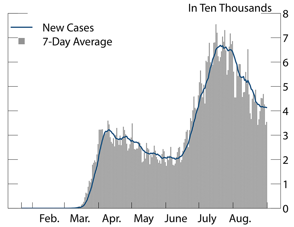
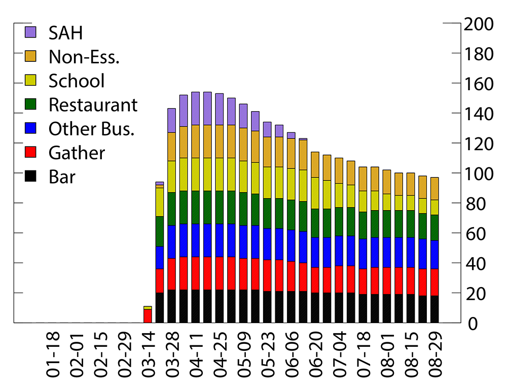
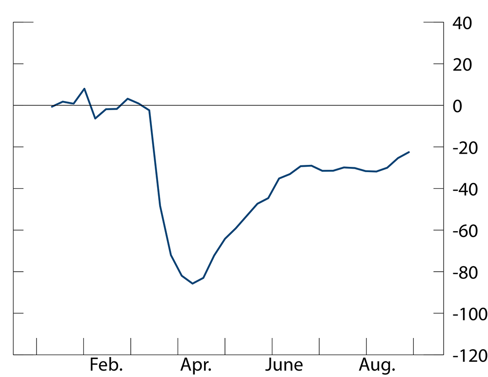
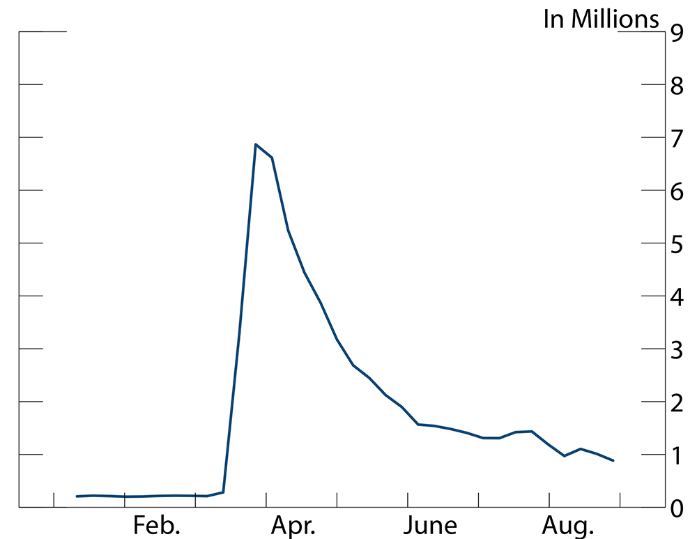
The first case of the coronavirus pandemic (COVID-19) in the United States was confirmed in mid-January, but the major outbreak was observed in mid-March reaching around 35,000 daily new cases by April 9. After the first wave of the pandemic subsided in May, the number of new cases started increasing again in June, reaching another yet higher peak in July and August (Figure 1, panel (a)). In an effort to contain the spread of the virus, nearly all states in the U.S. issued non-pharmaceutical interventions (NPIs)---such as stay-at-home orders and shutting down all nonessential businesses (Figure 1, panel (b)) and people responded by reducing their social interactions (Figure 1, panel (c)). At the same time, during the first wave, unemployment soared to a postwar record high when initial unemployment claims spiked in March and April, but gradually declined thereafter (Figure 1, panel (d)).
Figure 1 Panel (a), illustrates the daily new COVID-19 cases in United States (in bars) and 7-day moving averages in solid line from January 11, 2020 until August 29, 2020. Data source: Authors’ calculations based on data from the John’s Hopkins Coronavirus COVID-19 Global Cases Database. In Panel (b), we plot the total non-pharmaceutical interventions (NPIs) issued across all states in a given week. Source: Adolph et al. (2020). In Panel (c), we plot the national average Dallas FED Mobility and Engagement Index (MEI). Finally, in Panel (d), we show the weekly initial unemployment claims in millions from January 11, 2020 until August 29, 2020. Data source: FRED, St. Louis FED.
Figure 1a. COVID-19 cases

Figure 1b. Non-pharmaceutical interventions

Note. Categories are displayed in order from top to bottom. For March 14, only School and Gather appear
Source: Adolph et al. (2020).
Figure 1c. Mobility and Engagement Index

Figure 1d. Weekly U.S. initial claims

These observations raise a number of important questions: Did people reduce their social interactions as a result of the pandemic, restrictive lockdown policies, or both? What was the impact of reduced social interactions on local employment? Importantly, why did unemployment spike during the first wave of the pandemic, but gradually decline thereafter, even though the outbreak was much more severe during the second wave? Despite the policy relevance of these questions, the extant literature provides mixed conclusions.2
In this note, we attempt to answer these questions by exploiting newly available data on hours worked among small firms at the industry-county-state-week level. The granularity of the dataset allows us to saturate the model with different fixed effects, thereby controlling for confounding factors that hinder identification. For example, changes in mobility can be the result of both county-level pandemic intensity and state-level lockdown policies. Similarly, changes in local employment of nonessential industries can be the result of the shutdown of local businesses as well as reduced demand for nonessential goods and services, thus reducing demand for labor. As such, isolating the forces in action is warranted and is the main contribution of our note.
Our findings can be summarized as follows: In response to the pandemic, people have reduced mobility, which was more pronounced following state-wide imposed lockdown policies. Such effects of reduced mobility, especially due to stay-at-home orders and closure of non-essential businesses in the first wave, account for a substantial rise in unemployment across hourly workers, particularly those working in non-essential industries. From the set of workers that were laid off, only a small share found a new job in essential businesses, reducing the total local employment, especially during the first wave of the pandemic.
Unemployment data and descriptive analysis
To measure changes in employment, we use newly available weekly data on hours worked among employees of firms that use the Homebase software. Homebase data includes small and medium size enterprises (SMEs), with the majority of firms having fewer than 20 employees, and an average of seven employees. The sample coverage is limited to the SMEs that use the Homebase scheduling software. However, the data covers about 37,000 firms in January 2020, operating in all 50 states. Studying SMEs can shed light on important market developments. They generate about 44 percent of the overall U.S. economic activity (Kobe and Schwinn, 2018). SMEs, especially the ones relying on hourly workers, have been hit harder than larger companies because they typically have little or no equity, relying on financing via more bank loans with fewer debt instruments. Moreover, Homebase data allow us to observe employment of a firm throughout the time and enable us to study the impact of COVID-19 across counties and essential and non-essential industries.
Our sample includes the firms reporting data from January 11th, 2020 until August 29th, 2020.3 Table 1 provides the sample details. As of January 11th, 2020, before the outbreak of the pandemic, firms in our sample have about 160,000 hourly employees, spread across 2,276 counties in 50 states. As of end-of-April 2020, the number of employees halved compared to the pre-pandemic levels. Both essential and non-essential industries were affected greatly, with the impact being slightly higher for the non-essential ones. However, during the second wave, employment rebounded and leveled off at around 10 percent below the pre-pandemic level.
Table 1 shows the sample details of the Homebase data. In Panel A, we report the number of firms, employees, average hourly wages, mean and median number of employees for reporting firms for the entire sample, as well as for essential and non-essential businesses. In addition, we report the total number of counties and states present in the data. In Panel B, we list the industries included in the sample, their corresponding frequencies, and whether they are classified as essential or non-essential based on the Department of Homeland Security classification. For each of the statistics, we report the beginning of the sample, end of the first wave, and end of the second wave.
Table 1. Homebase data–sample details
Panel A.
| All firms | Firms in essential industries | Firms in nonessential industries | |||||||
|---|---|---|---|---|---|---|---|---|---|
| 2020w1 | 2020w16 | 2020w34 | 2020w1 | 2020w16 | 2020w34 | 2020w1 | 2020w16 | 2020w34 | |
| Number of firms | 37,140 | 37,140 | 37,140 | 34,887 | 34,887 | 34,887 | 2,253 | 2,253 | 2,253 |
| Number of employees | 159,423 | 76,474 | 141,918 | 153,058 | 73,560 | 135,588 | 6,365 | 2,914 | 6,330 |
| Average wage earned | 12.0 | 12.6 | 12.3 | 11.9 | 12.5 | 12.2 | 13.6 | 14.9 | 13.7 |
| Maximum employees | 288 | 178 | 235 | 288 | 178 | 235 | 104 | 85 | 84 |
| Median employees | 5 | 4 | 5 | 6 | 4 | 5 | 4 | 3 | 4 |
| Number of counties | 2,276 | 2,275 | 2,273 | 2,240 | 2,238 | 2,236 | 787 | 787 | 790 |
| Number of states | 50 | 50 | 50 | 50 | 50 | 50 | 50 | 50 | 50 |
Panel B.
| Category | Frequency of observations (%) | |||
|---|---|---|---|---|
| 2020w1 | 2020w16 | 2020w34 | ||
| Beauty and Personal Care | Non-essential | 1.11 | 1.11 | 1.11 |
| Charities, Education and Membership | Essential | 3.60 | 3.60 | 3.59 |
| Food and Drink | Essential | 54.87 | 54.88 | 54.89 |
| Health Care and Fitness | Essential | 9.42 | 9.41 | 9.40 |
| Home and Repair | Non-essential | 2.68 | 2.68 | 2.68 |
| Leisure and Entertainment | Non-essential | 2.25 | 2.25 | 2.25 |
| Professional Services | Essential | 4.60 | 4.60 | 4.60 |
| Retail | Essential | 20.44 | 20.44 | 20.43 |
| Transportation | Essential | 1.04 | 1.03 | 1.03 |
Data is grouped under nine industries, listed in Table 1, Panel B. Most of the firms operate under food and drink, followed by retail industries. We marked Beauty and Personal Care, Home and Repair, and Leisure and Entertainment industries as nonessential, per the Department of Homeland Security classification.4
Empirical analysis
We start by exploring the effects of community spread of the pandemic (COVID-19 deaths)5 and NPIs on the mobility patterns of the population. For identification, we exploit within-state-week variation across counties that are differently affected by the pandemic, thereby controlling for all observed and unobserved time-varying heterogeneity at the state level. We measure mobility using the Dallas FED Mobility and Engagement (MEI) Index. The MEI index captures valuable insights concerning mobility patterns and it is expected to inform responses against the COVID-19 pandemic. Formally, for state s, county c, and week t, we run the following panel regressions:
$$(1)\ \ \ \ \ \ \ \ \begin{array}{ll}\mathrm{MEI}_{s, c, t+1}= & \beta_{1} \mathrm{Deaths}_{c, t} \times D1_t+\beta_{2} \mathrm{Deaths}_{c, t} \times D2_t+ \\ & \gamma_{1} \mathrm{Deaths}_{c, t} \times \mathrm{NPIs}_{s, t} \times D 1_{t}+\gamma_{2} \mathrm{Deaths}_{c, t} \times \mathrm{NPIs}_{s, t} \times D2_{t}+ \\ & \eta_{s} \times v_{t}+\rho_c+\varepsilon_{s, c, t}\end{array}$$
$$\mathrm{Deaths}$$ is the county level COVID-19 deaths per capita from the Johns Hopkins Coronavirus COVID-19 Global Cases Database. $$\mathrm{NPIs}$$ are the state-level social distancing policies in response to the pandemic, from Adolph et al. (2020). We particularly focus on the stay-at-home orders and nonessential business closures. $$D1$$ is a dummy variable, which is equal to 1 in the first wave of the pandemic (2020/01/11–2020/05/30). Similarly, $$D2$$ equals 1 in the second wave of the pandemic (2020/06/06–2020/08/29). Finally, $$\eta_s$$, $$v_t$$, and $$\rho_c$$ are the state, week, and county fixed effects, respectively. State×time fixed effects are essential as they fully capture the time-varying state-level characteristics such as state level economic activity and demographics. We clustered the standard errors at the state-week level.
In Table 2, we find that a one standard deviation increase in deaths per-capita was associated with about one percent decrease in mobility. We also find that the reduction in county mobility was more pronounced after a state-wide stay-at-home order was enacted. Comparing the first two waves of the pandemic, we find that the impact of NPIs on mobility was more than four times higher during the first wave compared to the second wave. Given a level of deaths per-capita, a one-week lengthening of a stay-at-home order decreased mobility by 2.5 percent during the first wave, whereas it decreased by only 0.6 percent in the second wave. Similar conclusions arise when we use the closure of non-essential businesses instead of stay-at-home orders (Column 3). Thus, the main underlying reason of the reduced mobility was the aggressively implemented NPIs, rather than the fear caused by the community spread of the pandemic.
Table 2 reports the estimated coefficients of panel regressions introduced in (1), which regresses the Dallas FED Mobility and Engagement Index (MEI) index on per-capita COVID-19 deaths in county c in week t. County level deaths are obtained from the Johns Hopkins Coronavirus COVID-19 Global Cases Database. Non-pharmaceutical interventions (NPIs) are the state-level stay-at-home orders introduced in response to the pandemic, from Adolph et al. (2020). In column 1, we report the effects of deaths per-capita on the mobility of the population during the first wave of the pandemic (2020/01/11–2020/05/30) and the second wave of the pandemic (2020/06/06–2020/08/29) separately. In addition to deaths per-capita, in columns 2 and 3, we include stay-at-home orders and closure of non-essential businesses as NPIs, respectively. In all of the specifications, standard errors are clustered at the state-week level and all variables are standardized to ease the interpretation of the estimated coefficients. Fixed effects used in the specifications are listed at the bottom of the table and not presented for the sake of brevity. ***, **, and * denote significance at the 1%, 5%, and 10% level (two-sided), respectively.
Table 2. The impact of pandemic intensity and NPIs on mobility
| Dep: MEI$$_{t+1,c}$$ | 1 | 2 | 3 |
|---|---|---|---|
| Wave 1: Per-capita COVID-19 deaths$$_{t,c}$$ | -1.09*** | -0.60*** | -0.49*** |
| (0.110) | (0.069) | (0.071) | |
| Wave 2: Per-capita COVID-19 deaths$$_{t,c}$$ | -0.91*** | -0.90*** | -0.65*** |
| (0.133) | (0.128) | (0.093) | |
| Wave 1: NPI$$_{t,s}$$ | -0.74*** | -0.83*** | |
| (0.125) | (0.151) | ||
| Wave 2: NPI$$_{t,s}$$ | -0.18*** | -0.43** | |
| (0.030) | (0.172) | ||
| County FE | yes | yes | yes |
| State $$\times$$ Week FE | yes | yes | yes |
| Observations | 74,511 | 74,511 | 74,511 |
| adjR2 | 0.939 | 0.939 | 0.939 |
Having established the strong relationship between the COVID-19 deaths per-capita, NPIs, and mobility, we then turn to the effects of the pandemic on employment, using the mobility as a measure of the county-level pandemic intensity. Being highly correlated with the number of deaths and the NPIs, mobility arguably indicates a more comprehensive geographic effect of the pandemic.
Estimating adjustments in employment during a pandemic poses a key identification challenge. Employment can adjust either due to reduced labor force amid COVID-19 cases and deaths or weaker demand for goods and services due to NPIs and mobility, particularly for nonessential businesses. To distinguish between alternative channels, our specifications include two set of fixed effects that are crucial for identification. On the one hand, the set of county-week fixed effects allows us to study the employment dynamics of essential versus nonessential industries that operate within the same county and week, thereby controlling for all observed and unobserved time-varying heterogeneity at the county level. This includes pandemic intensity or policies to mitigate the impact of the pandemic at the county-level. On the other hand, the set of industry-state-week fixed effects allows us to study the employment dynamics of the same industry that operates across counties within the same state and week, thereby controlling for all observed and unobserved time-varying heterogeneity at the industry-state level. This includes state-wide lockdown policies or the overrepresentation of some industries in certain states (e.g., financial services in New York, manufacturing in Michigan). Taken together, we exploit these two sources of variation at the same time to analyze the impact of reduced mobility on the employment dynamics of essential versus nonessential industries. Formally, for industry $$i$$, state $$s$$, county $$c$$, and week $$t$$, we run the following panel regressions:
$$(2)\ \ \ \ \ \ \ \ \begin{array}{ll}\Delta \mathrm{logEmployment}_{i, s, c, t+1}= & \beta_{1} \mathrm{MEI}_{c, t} \times \text{Non-essential}_i \times D1_t + \\ & \beta_2 \mathrm{MEI}_{c, t} \times \text{Non-essential}_i \times D2_t + \rho_c \times v_t + \kappa_i \times \eta_s \times v_t + \varepsilon_{i,s,c,t}, \end{array}$$
where, $$\Delta\mathrm{logEmployment}$$ is the log change of total employment in week $$t$$, compared to the first week of January 2020 and $$\mathrm{MEI}$$ is the county level, weekly mobility and engagement index. $$\text{Non-essential}$$ is a dummy equal one if an industry is classified as non-essential based on the Department of Homeland Security classification. $$D1$$ is a dummy variable, which is equal to 1 in the first wave of the pandemic (2020/01/11– 2020/05/30). Similarly, $$D2$$ equals 1 in the second wave of the pandemic (2020/06/06– 2020/08/29). Finally, $$\eta_s$$, $$v_t$$, $$\rho_c$$, and $$\kappa_i$$ are the state, week, county, and industry fixed effects, respectively.
We find that lower mobility was associated with a significant reduction in employment of nonessential businesses, compared to the essential businesses throughout the sample period (Table 3, column 1). We find strong effects of mobility restriction contributing to an increase in unemployment during the first wave and a lesser impact during the second wave. This provides supporting evidence that the unprecedented drop in employment during the first wave was mainly driven by the sharp drop in mobility of people, which was in turn due to the aggressive implementation of the NPIs.
Table 3 reports the estimated coefficients of panel regressions in (2). The dependent variable, ∆log(Employment)t+1,c, is the log change of total employment, against the first week of 2020, which we use as benchmark. MEIt,c is the Dallas FED Mobility and Engagement Index for county c in week t. Non-pharmaceutical interventions (NPIs) are the state-level stay-at-home orders introduced in response to the pandemic, from Adolph et al. (2020). The first wave of the pandemic (2020/01/11– 2020/05/30) and the second wave of the pandemic (2020/06/06–2020/08/29) are reported separately. Non-essential and essential industries are listed in Table 1. In all specifications, standard errors are clustered at the state-week level and all variables are standardized to ease the interpretation of the estimated coefficients. Fixed effects used in the specifications are listed at the bottom of the table and not presented for the sake of brevity. ***, **, and * denote significance at the 1%, 5%, and 10% level (two-sided), respectively.
Table 3. Impact of COVID-19 on employment
| Dep: $$\Delta \log \text{(Employment)}_{t+1,c}$$ | 1 | 2 | 3 | 4 |
|---|---|---|---|---|
| MEI $$\times \text{Non-Essential Industry}_{t,c}$$ | 0.11*** | |||
| (0.010) | ||||
| Wave 1: MEI $$ \times \text{Non-Essential Industry}_{t,c}$$ | 0.11*** | |||
| (0.011) | ||||
| Wave 2: MEI $$\times \text{Non-Essential Industry}_{t,c}$$ | 0.04*** | |||
| (0.008) | ||||
| NPI$$_{t,s}$$ | 0.05*** | |||
| (0.006) | ||||
| Wave 1: NPI$$_{t,s}$$ | 0.06*** | |||
| (0.007) | ||||
| Wave 2: NPI$$_{t,s}$$ | 0.03*** | |||
| (0.004) | ||||
| County $$\times$$ Week FE | yes | yes | no | no |
| Industry $$\times$$ State $$\times$$ Week FE | yes | yes | no | no |
| County FE | no | no | yes | yes |
| State $$\times$$ Week FE | no | no | yes | yes |
| Observations | 159,552 | 159,552 | 69,991 | 69,991 |
| adjR2 | 0.536 | 0.536 | 0.672 | 0.672 |
Finally, we examine the possible reallocation of employees between the essential and nonessential industries. It is argued in the literature that the pandemic forces the rapid reallocation of labor, with companies and governments mobilizing an army of idled workers into new activities that are urgently needed (See for e.g., Bender and Dalton, 2020). Barrero et al. (2020) provide supporting evidence of such reallocation at the early stages of the pandemic. If all of the workers that were laid off from nonessential businesses found a new job in essential businesses, then the effect on total employment at the county-level would be zero. To this end, we aggregate our county-state-week-industry level data to the county-state-week level, and then regress changes in weekly employment with respect to the employment level in the first week of January on MEI. Exploiting within-state-week variation, in Table 3, columns 3 and 4, we find evidence of partial reallocation of workers from nonessential to essential businesses, especially during the second wave.
References
Abouk, R. and B. Heydari (2021). The immediate effect of covid-19 policies on socialdistancing behavior in the united states. Public Health Reports 136(2), 245–252.
Adolph, C., K. Amano, B. Bang-Jensen, N. Fullman, and J. Wilkerson (2020). Pandemic politics: Timing state-level social distancing responses to covid-19.Journal of Health Politics, Policy and Law Sep 16:8802162 .
Baek, C., P. B. McCrory, T. Messer, and P. Mui (2020). Unemployment effects of stay-at-home orders: Evidence from high frequency claims data. Review of Economics and Statistics forthcoming, 1–72.
Barrero, J. M., N. Bloom, and S. J. Davis (2020). Covid-19 is also a reallocation shock. Technical report, National Bureau of Economic Research.
Bartik, A. W., M. Bertrand, F. Lin, J. Rothstein, and M. Unrath (2020). Measuring the labor market at the onset of the covid-19 crisis. Technical report, National Bureau of Economic Research.
Bender, R. and M. Dalton (2020). Coronavirus pandemic compels historic labor shift: Outbreak reshapes job market as some sectors shut down, other see demand surge. Wall Street Journal 29.
Correia, S., S. Luck, and E. Verner (2020). Pandemics depress the economy, public health interventions do not: Evidence from the 1918 flu.
Kobe, K. and R. Schwinn (2018). Small business gdp 1998-2014.
Maloney, W. and T. Taskin (2020). Determinants of social distancing and economic activity during covid-19: A global view. The World Bank Policy Research Working Papers 9242.
1. Federal Reserve Board. The views in this paper are solely those of the authors and should not be interpreted as reflecting the views of the Board of Governors of the Federal Reserve System or of any other person associated with the Federal Reserve System. Return to text
2. For example, Abouk and Heydari (2021) find that statewide NPIs had strong causal impacts on reducing social interactions, while Maloney and Taskin (2020) find that the increase in social distancing was largely voluntary. Focusing on employment, Baek et al. (2020) show that about a quarter of the initial unemployment claims at the beginning of the pandemic can be attributed to the stay-at-home orders. Return to text
3. The number of firms in the sample fluctuates as some firms exit when they stop using the software (either due to business closure or terminating their contract with Homebase) or enter into the sample (either due to business opening or entering an agreement with Homebase). To avoid the survivorship bias, we only keep firms that report during the whole sample. Return to text
4. https://www.cbia.com/resources/coronavirus/coronavirus-state-federal-updates/department-homeland-security-essential-industries/ Return to text
5. We use deaths per-capita instead of cases per-capita as number of cases are highly dependent on the number of available tests. Such argument is particularly important given that the available testing was highly limited in the first wave of the pandemic. We test the sensitivity of our results and conclude that the main findings hold when cases per-capita is used instead. Return to text
Dockerty, J. Marcus, Antonis Kotidis, and Ilknur Zer (2021). "How much lockdown policies contribute to local unemployment? Evidence from the first and second waves of COVID-19," FEDS Notes. Washington: Board of Governors of the Federal Reserve System, May 24, 2021, https://doi.org/10.17016/2380-7172.2903.
Disclaimer: FEDS Notes are articles in which Board staff offer their own views and present analysis on a range of topics in economics and finance. These articles are shorter and less technically oriented than FEDS Working Papers and IFDP papers.