FEDS Notes
March 08, 2024
Measuring Unemployment Risk
Brendan J. Chapuis and John Coglianese
Introduction
In this note, we introduce a measure of unemployment risk, the likelihood of a worker becoming unemployed within the next twelve months. By using nonparametric machine learning applied to data on millions of workers in the US, we can estimate how unemployment risk varies across individuals and over time. We validate our estimates by showing that patterns of ex ante unemployment risk mirror those of ex post unemployment, including stark differences across demographic groups and duration dependence among the unemployed. Using our estimates, we find that unemployment risk is highly concentrated, particularly among individuals who are currently unemployed but also in the tails of the distributions for employed and not-in-the-labor-force individuals. During recessions, unemployment risk surges, driven largely but not completely by those currently unemployed.
An important advantage of our approach is that we can measure unemployment risk faced by workers who have yet to become unemployed. Among the employed, we find that the distribution of unemployment risk is highly unequal, with highly exposed workers having a nearly 10 times greater likelihood of future unemployment than less exposed workers. This ratio remains roughly constant over the business cycle, such that as unemployment risk rises in aggregate during a recession, the most exposed workers see substantially higher increases in the level of risk they face. This heterogeneity is especially pronounced across industries, with more cyclically sensitive industries having a greater difference in the unemployment risk faced by their most and least exposed workers.
Our measure of unemployment risk can be a helpful tool for understanding the labor market, examining consumer behavior, and guiding policy. We provide estimates of the margins along which unemployment rises in recessions, not only by breaking down the contributions of different labor force statuses as in Shimer (2012), Elsby et al. (2009), and Elsby et al. (2015), but also by measuring the change in the distribution within these groups. Our measure may also be useful beyond the labor market context, for example in understanding the incentives different households have to engage in precautionary savings behavior over the business cycle as in Ravn and Sterk (2017) and Bayer et al. (2019). Lastly, our results highlight that some workers face substantially higher risk of unemployment than others, which raises the value of unemployment insurance (among other safety net policies) for these workers.
Measuring Unemployment Risk
Methodology
We define unemployment risk for individual $$ i $$ in time period $$t$$ as the probability of unemployment twelve months into the future,
$$$$ \text{Unemployment Risk}_{i,t} \equiv \Pr\left(U_{i,t+12} | X_{i,t} \right) $$$$
where $$U_{i,t+12}$$ is an indicator for future unemployment, $$X_{i,t}$$ is a vector of individual characteristics, including labor force status, demographic information, and job characteristics (if employed).1 By including many dimensions of information about the individual in $$X_{i,t}$$, our approach nests several different breakdowns of unemployment. Previous work has highlighted differences across education levels (Jefferson, 2008), racial groups (Cajner et al., 2017), and the age distribution (Hoynes et al., 2012). Our approach nests each of these breakdowns and allows for potentially nonlinear interactions between different dimensions.
We estimate unemployment risk as a function of individual characteristics using a nonparametric machine learning algorithm fit to data on realized unemployment outcomes. We use the method of gradient boosting classification trees since this is particularly well-suited for estimating probabilities as a flexible function of many continuous and discrete dimensions, allowing for arbitrary interactions and nonlinearities along each dimension.2 This method is widely used in machine learning for so-called "tabular" data and has been found to be among the best performing methods in a variety of settings (Shwartz-Ziv and Armon, 2022; Grinsztajn et al., 2022; Gu et al., 2020; Cengiz et al., 2022). By using data on realized unemployment outcomes, we are estimating unemployment risk for the population that our sample was drawn from, but different populations (e.g. other countries or eras) may have different distributions of unemployment risk.3
By looking twelve months into the future, our measure of unemployment risk combines risks of unemployment from different types of transitions. For example, our measure of unemployment risk for a worker who is currently employed combines both the likelihood of separation from her current job as well as the likelihood of not finding a new job by twelve months in the future. In this way, we combine heterogeneity in separation rates and job finding rates (and other transition rates) into a single measure for each individual. We view this approach as more comprehensive than examining heterogeneity in specific transition rates in isolation.
With an estimate of the unemployment risk function, we can measure how unemployment risk varies across groups and over time. For each individual in our sample, we use the estimated function mapping characteristics into probabilities of future unemployment to calculate that individual's estimated unemployment risk. We use survey weights to aggregate these unemployment risk values to the subgroup or overall population level in order to ensure that the statistics we calculate are representative of the U.S. population.
Data
To estimate unemployment risk, we use IPUMS Current Population Survey (CPS) microdata files from 2000 to 2023, which include a variety of demographic, economic, and labor variables for individuals and households (Flood et al., 2023). For each individual in the data, we establish a longitudinal link for their responses in each month (Rivera Drew et al., 2014), which we then use to generate a 12-month leading unemployment indicator for individuals who can be linked. We verify these matches by validating on demographic variables (Madrian and Lefgren, 2000). We drop from the sample individuals who cannot be linked over twelve months, as well as individuals less than 16 years old and those without labor force information.
We estimate unemployment risk in our sample as a function of many individual-level characteristics. We include current employment status characteristics (employed/unemployed/not in the labor force, unemployment duration, work absence, reason for unemployment, reason for non-participation), demographic characteristics (age, education, race, ethnicity, sex, disability, nativity, citizenship, marital status, number of children, family income), job characteristics (occupation, industry, professional certification, paid hourly, part-time or full-time, hours worked last week), and geographic characteristics (state, metropolitan area code, metropolitan area status). We also include the response date and calendar month.4 In addition to these individual characteristics, we include with each observation the current state-level unemployment rate and lagged 12-month changes in the state unemployment rate (from BLS Local Area Unemployment Statistics), as well as lagged 12-month percent changes in state-level employment and state-by-industry employment for the relevant industry (from the Quarterly Census of Employment and Wages).
We use a data-driven approach to tune our estimator for unemployment risk. We conduct a grid search to determine the optimal combination of parameters for gradient boosting classification trees in this setting (Ke et al., 2017). This grid search focuses on three parameters: the learning rate, the number of iterations (or trees), and the number of leaves per tree. For each step of the grid search, we use five-fold cross-validation to estimate out-of-sample prediction error in terms of average root mean squared error (RMSE) for the holdout sample. We choose the set of parameters which minimize average RMSE as the optimal parameters and then re-train the model on the entire sample using these parameters. With the model trained, we then apply it to the data and predict unemployment risk for all individuals in our sample. To estimate statistics for unemployment risk (e.g. average unemployment risk by subgroup), we use CPS microdata weights to account for sampling probability.
Validating our Measure of Unemployment Risk
We begin by examining whether our measure of unemployment risk features similar patterns as realized unemployment.
Unemployment varies substantially across demographic groups, and unemployment risk mirrors these differences. Figure 1 reports the average value of unemployment risk over 2000-2022 for separate groups by gender, education, race, and nativity, along with the average unemployment-to-population ratio for each group.5
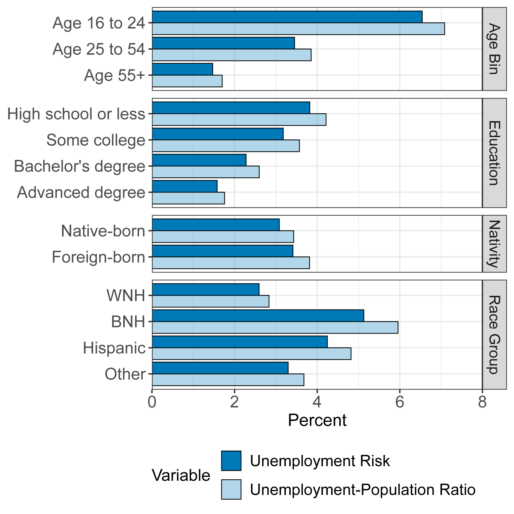
Notes: This figure shows average unemployment risk in our sample broken down for different demographic groups. Statistics are calculated from the Current Population Survey (CPS), using the subsample of respondents that can be matched over twelve months. This subsample includes approximately 2.85 million respondents over 2000-2022. Unemployment risk is measured using estimates from Equation 1 applied to the subsample. Unemployment-to-population ratio differs from the conventional unemployment rate in dividing by population instead of labor force. "WNH" and "BNH" refer to white non-Hispanic and Black non-Hispanic, respectively.
Our measure of unemployment risk is also able to replicate the well-documented pattern of duration dependence in unemployment. Figure 2 plots the average unemployment risk of currently-unemployed individuals with different durations of their current spell for an expansionary year (2007) and a recessionary year (2009). In both years, longer durations see higher levels of future unemployment risk. In 2009, after the recession had occurred, unemployment risk goes up for all durations but especially for those beyond 6 months. It is important to note that the duration dependence in unemployment risk we identify could result from either a causal effect of duration (Kroft et al., 2013) or heterogeneity among unemployed workers (Ahn and Hamilton, 2020), but our approach does not distinguish between these explanations.
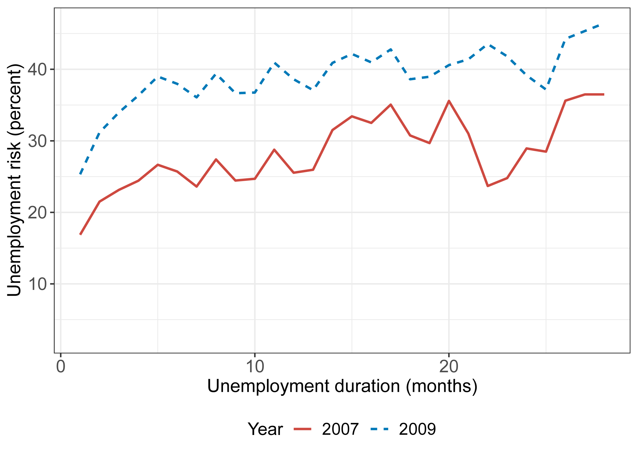
Notes: This figure shows average unemployment risk for the unemployed broken down by duration for years before and after the Great Recession. Statistics are calculated from the Current Population Survey (CPS), using the subsample of respondents that can be matched over twelve months who were initially unemployed in either 2007 or 2009. This subsample includes 7,859 respondents in 2007 and 13,659 respondents in 2009. Unemployment risk is measured using estimates from Equation 1 applied to the subsample for each year. We convert unemployment duration in weeks to months by dividing by 4.33 and rounding.
Inequality of Unemployment Risk
Figure 3 illustrates how unemployment risk shifts across labor force categories over the business cycle. We discuss each of the components of this shift in turn.
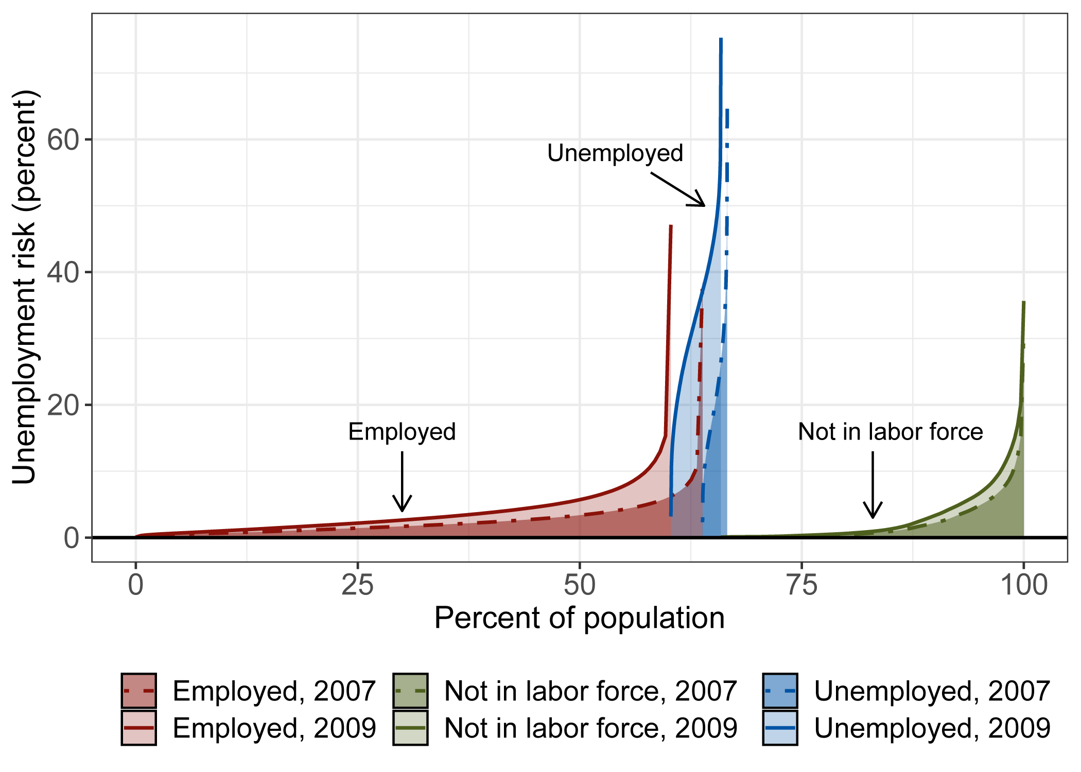
Notes: This figure shows the distributions of unemployment risk for years before and after the Great Recession, where we calculate the distribution separately for each main labor force status category. Statistics are calculated from the Current Population Survey (CPS), using the subsample of respondents that can be matched over twelve months who initially responded in either 2007 or 2009. This subsample includes 160,602 respondents in 2007 and 164,788 respondents in 2009. Unemployment risk is measured using estimates from Equation 1 applied to the subsample for each year. Within each labor force status category, we rank individuals by unemployment risk for each year, and the horizontal span of the distribution corresponds to the population share of that category.
Before a recession, unemployment risk is relatively concentrated. The dashed lines in Figure 3 show the distribution of unemployment risk as of 2007 broken out separately for employed, unemployed, and not-in-the-labor-force individuals. Unemployment risk was below 5% for the vast majority of employed workers, and below 10% for all but the extreme tail. Since the unemployment rate was low in 2007, unemployed workers made up only a small sliver of the population (2.8%), but this group had an average unemployment risk of nearly 22%, about ten times larger than either of the other categories (2.7% average for employed, 2.4% average for not in the labor force).
During a recession, unemployment risk increases across the distribution, especially for the unemployed. The solid lines in Figure 3 show unemployment risk for each category as of 2009, which increased from 2007 at every percentile. The unemployed experienced a particularly large increase in average unemployment risk, jumping from 22% in 2007 to 33% in 2009, but there were also meaningful increases for the employed (from 2.7% to 3.9%) and not in the labor force (from 2.4% to 3.2%).
In addition to increased unemployment risk within each group, the large surge of unemployment in the labor market meant that relatively fewer individuals were in the lower unemployment risk groups (employed and not in the labor force) compared to the 2007 distribution. Between 2007 and 2009, the increase in average unemployment risk for the unemployed (from 22% to 33%) and the increase in the population share of this category (from 2.8% to 5.6%) combined to more than triple the contribution of this group to average unemployment risk for the total population.
Beyond the central role of the unemployed in driving unemployment risk during recessions, we also find a modest contribution for increased unemployment risk among the employed. Among the set of workers who still had jobs in 2009, higher unemployment risk could reflect either higher expected separation rates or lower job-finding rates conditional on separating, or some combination of these factors (Shimer, 2012). Despite the decrease in the population share of the employed, the increase in unemployment risk among this group is large enough to account for roughly one quarter of the population-wide increase in unemployment risk.
Among employed workers, unemployment risk is highly unequal. Figure 4 shows the distribution of log unemployment risk among the employed for a selection of years. Compared to workers at the 10th percentile, workers at the 90th percentile are typically about 2.3 log points, or roughly 10 times, more likely to become unemployed within the next year.
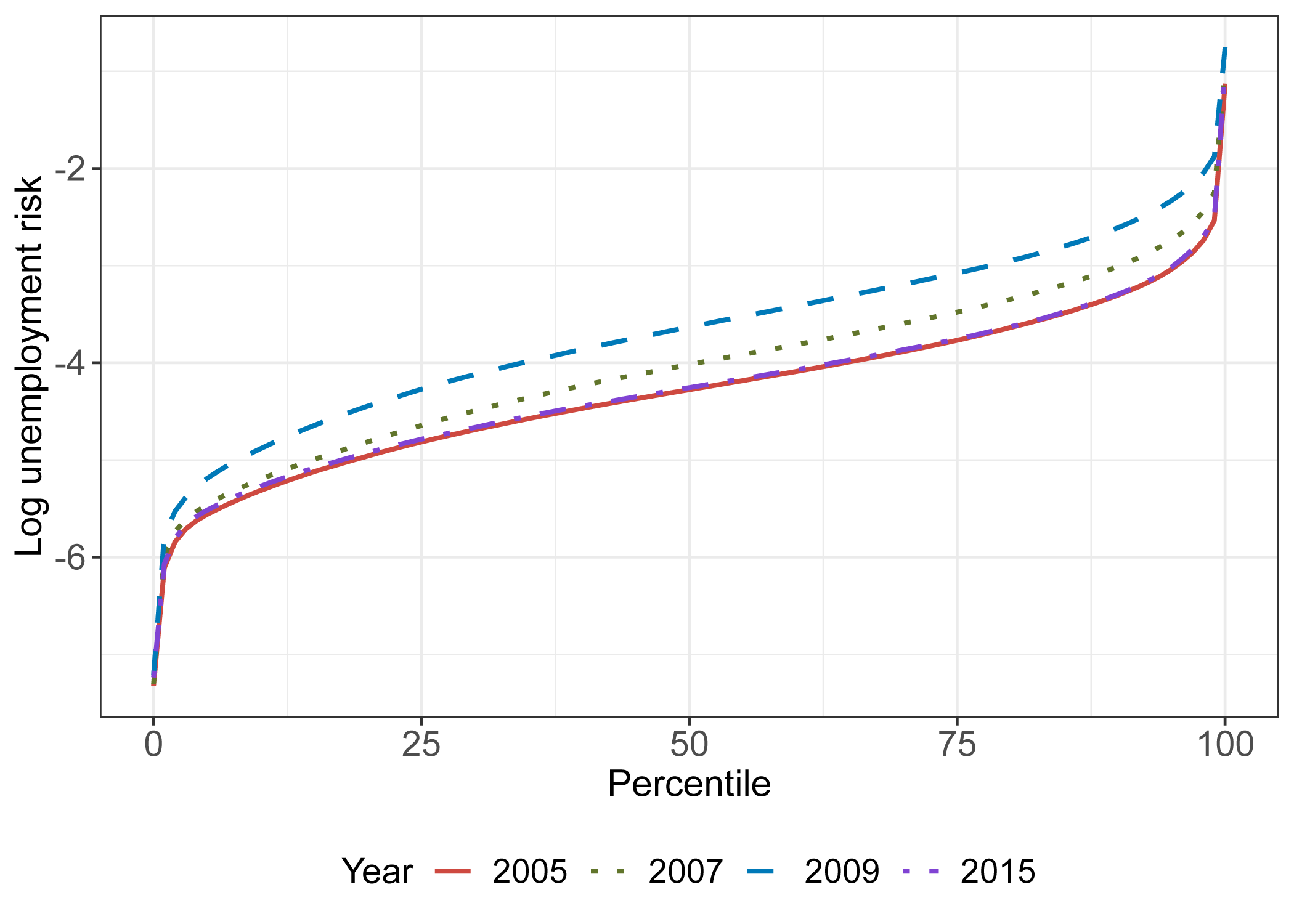
Notes: This figure shows the distribution of log unemployment risk among employed individuals for years before and after the Great Recession. Statistics are calculated from the Current Population Survey (CPS), using the subsample of respondents that can be matched over twelve months who initially responded in either 2005, 2007, 2009, or 2015. This subsample includes 160,420 respondents in 2005, 160,602 respondents in 2007, 164,788 respondents in 2009, and 159,016 respondents in 2015. Unemployment risk is measured using estimates from Equation 1 applied to the subsample for each year.
Among the employed, shifts in unemployment risk over the business cycle are remarkably consistent. The distributions for the years before, during, and after the Great Recession shift by roughly similar amounts at each percentile, with the exceptions of the extreme tails. It is important to note that with the log scale constant unit changes represent multiplicative changes in unemployment risk rather than additive changes. From 2005 to 2009, log unemployment risk shifts up by about 0.7 log points for most percentiles, or roughly a doubling of unemployment risk in levels, and shifts back down by the same amount by 2015.
Within the group of employed workers, changes in unemployment risk over the business cycle are much larger for cyclically-exposed industries. Figure 5 illustrates how unemployment risk varies within several industries, showing the evolution of the 25th and 75th percentiles of unemployment risk within these industries. For the 75th percentile workers, there are large differences both across industries and over the business cycle. The 75th percentile for construction workers peaks at about 12% in 2008, approximately double the values for manufacturing or retail trade that year and nearly quadruple the value for professional & related services. The ordering of the 75th percentile across industries is the same for most years, with construction the highest followed by retail trade and then manufacturing, but there are notable exceptions such as the pandemic period when retail trade eclipses the other industries.
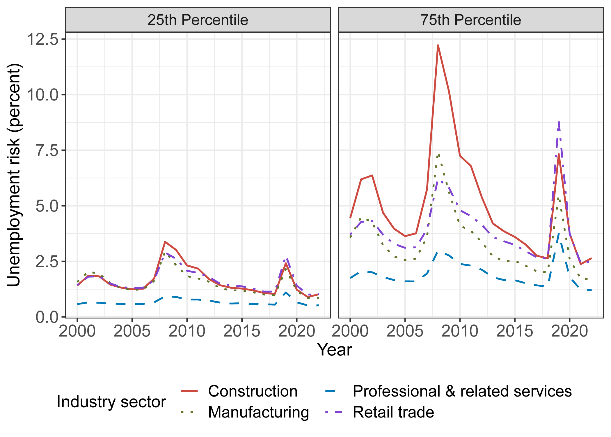
Notes: This figure shows the 25th and 75th percentile of unemployment risk within a subset of large industries over time. Statistics are calculated from the Current Population Survey (CPS), using the subsample of respondents that can be matched over twelve months who initially responded as being employed in either construction, professional & related services, manufacturing, or retail trade. These four industries account for 62.9 percent of employed individuals in the sample and 38.5 percent of total individuals in the sample. Unemployment risk is measured using estimates from Equation 1 applied to the subsample for each industry. For each industry and year, we rank individuals by unemployment risk and report the 25th and 75th percentiles.
In contrast, workers less exposed to the business cycle within each industry experience more similar evolution of unemployment risk. For 25th percentile workers, all industries show fairly low levels of unemployment risk, consistently below 4% each year with relatively small cyclical fluctuations (especially so for professional & related services). 25th percentile workers in construction, manufacturing, and retail trade experience similar unemployment risk as 75th percentile workers in professional & related services.
Conclusion
We introduce a measure of unemployment risk, defined as the likelihood of a worker being unemployed 12 months from now, and estimate the distribution of unemployment risk using a machine learning method applied to CPS microdata. While our measure of unemployment risk aligns with measures of ex post unemployment across various dimensions, a key advantage of our measure is that it can be used to assess ex ante risk for all individuals, including for those who are currently employed. We find that unemployment risk is concentrated not only among the unemployed, but also in the tails of the distribution for the employed and those not in the labor force. Over the business cycle, the unemployment risk of the most exposed workers is consistently about 10 times greater than the risk of the least exposed workers, and a similar heterogeneity of risk is also observed across industries. This measure of unemployment risk yields valuable insights about the distribution of risk within labor markets, making it a helpful tool both for future research and policy.
References
Ahn, H. J., & Hamilton, J. D. (2020). Heterogeneity and unemployment dynamics. Journal of Business & Economic Statistics, 38(3), 554-569.
Bayer, C., Lütticke, R., Pham‐Dao, L., & Tjaden, V. (2019). Precautionary savings, illiquid assets, and the aggregate consequences of shocks to household income risk. Econometrica, 87(1), 255-290.
Cajner, T., Radler, T., Ratner, D., & Vidangos, I. (2017). Racial gaps in labor market outcomes in the last four decades and over the business cycle. FEDS Working Paper.
Cengiz, D., Dube, A., Lindner, A., & Zentler-Munro, D. (2022). Seeing beyond the trees: Using machine learning to estimate the impact of minimum wages on labor market outcomes. Journal of Labor Economics, 40(S1), S203-S247.
Elsby, M. W., Hobijn, B., & Şahin, A. (2015). On the importance of the participation margin for labor market fluctuations. Journal of Monetary Economics, 72, 64-82.
Elsby, M. W., Michaels, R., & Solon, G. (2009). The ins and outs of cyclical unemployment. American Economic Journal: Macroeconomics, 1(1), 84-110.
Flood, S., King, M., Rodgers, R., Ruggles, S., Warren, J. R., Backman, D., . . . Westberry, M. (2023). IPUMS CPS: Version 11.0. Minneapolis, MN: IPUMS. Retrieved from https://doi.org/10.18128/D030.V11.0
Friedman, J. H. (2001). Greedy function approximation: a gradient boosting machine. Annals of Statistics, 1189-1232.
Friedman, J. H. (2002). Stochastic gradient boosting. Computational Statistics & Data Analysis, 38(4), 367-378.
Grinsztajn, L., Oyallon, E., & Varoquaux, G. (2022). Why do tree-based models still outperform deep learning on typical tabular data? Advances in Neural Information Processing Systems, 35, 507-520.
Gu, S., Kelly, B., & Xiu, D. (2020). Empirical asset pricing via machine learning. The Review of Financial Studies, 33(5), 2223-2273.
Hastie, T., Tibshirani, R., & Friedman, J. H. (2009). The Elements of Statistical Learning: Data Mining, Inference, and Prediction (Vol. 2). New York: Springer.
Hoynes, H., Miller, D. L., & Schaller, J. (2012). Who suffers during recessions? Journal of Economic Perspectives, 26(3), 27-48.
Jefferson, P. N. (2008). Educational attainment and the cyclical sensitivity of employment. Journal of Business & Economic Statistics, 26(4), 526-535.
Ke, G., Meng, Q., Finley, T., Wang, T., Chen, W., Ma, W., . . . Liu, T.-Y. (2017). Lightgbm: A highly efficient gradient boosting decision tree. Advances in Neural Information Processing Systems, 30.
Kroft, K., Lange, F., & Notowidigdo, M. J. (2013). Duration dependence and labor market conditions: Evidence from a field experiment. The Quarterly Journal of Economics, 128(3), 1123-1167.
Madrian, B. C., & Lefgren, L. J. (2000). An approach to longitudinally matching Current Population Survey (CPS) respondents. Journal of Economic and Social Measurement, 26(1), 31-62.
Ravn, M. O., & Sterk, V. (2017). Job uncertainty and deep recessions. Journal of Monetary Economics, 90, 125-141.
Rivera Drew, J. A., Flood, S., & Warren, J. R. (2014). Making full use of the longitudinal design of the Current Population Survey: Methods for linking records across 16 months. Journal of Economic and Social Measurement, 39(3), 121-144.
Shimer, R. (2012). Reassessing the ins and outs of unemployment. Review of Economic Dynamics, 15(2), 127-148.
Shwartz-Ziv, R., & Armon, A. (2022). Tabular data: Deep learning is not all you need. Information Fusion, 81, 84-90.
1. Since $$U_{i,t+12}$$ is defined for all individuals, not just those currently in the labor force, the average level of $$\text{Unemployment Risk}_{i,t}$$ will be roughly equivalent to the unemployment-to-population ratio rather than the conventional unemployment rate. Return to text
2. The gradient boosting trees method was developed Friedman (2001) and Friedman (2002); see Hastie et al. (2009) for an overview. Return to text
3. Relatedly, our measure of unemployment risk is conditional on macroeconomic developments that occurred during our sample period. A broader measure of unemployment risk would also include, for example, the likelihood of a recession within the next twelve months. Return to text
4. For calendar month, we include a trigonometric representation to account for the fact that seasonal effects can "wrap around" from one year to the next. Specifically, we number months $$m\in\{1,...,12\}$$ and we include $$m_A = sin(2\pi\frac{i}{12})$$ and $$m_B = cos(2\pi\frac{i}{12})$$. Return to text
5. We use the unemployment-to-population ratio instead of the conventional unemployment rate to have consistent levels with our measure of unemployment risk. Return to text
Brendan J. Chapuis and John Coglianese (2024). "Measuring Unemployment Risk," FEDS Notes. Washington: Board of Governors of the Federal Reserve System, March 08, 2024, https://doi.org/10.17016/2380-7172.3453.
Disclaimer: FEDS Notes are articles in which Board staff offer their own views and present analysis on a range of topics in economics and finance. These articles are shorter and less technically oriented than FEDS Working Papers and IFDP papers.