Board of Governors of the Federal Reserve System

March 31, 2025

Monetary Policy and the Distribution of Income: Evidence from U.S. Metropolitan Areas¹

Giovanni Favara, Francesca Loria, Gregory Marchal, and Egon Zakrajšek

The steady rise in income inequality and the broad range of actions undertaken by central banks in recent years – first to stabilize the global economy during the 2008-09 financial crisis and second to stave off the pandemic-induced economic collapse – have brought the distributional footprint of monetary policy to the forefront of the economic policymaking discussion (Bernanke, 2015; Draghi, 2016; BIS, 2021). From a theoretical perspective, understanding the redistributive channels through which monetary policy operates and transmits to the real economy is important to enhance the design of macroeconomic stabilization policies and ensure higher prosperity for the economy as a whole (Kaplan et al., 2018; Auclert, 2019).

Even so, empirical analysis on this subject, especially for the United States, is scant, in large part due to challenges in obtaining data that enable such analysis. Longitudinal U.S. household income data that span many years are rarely available, while surveys of U.S. household income can suffer from bias due to under-reporting and missing responses. Moreover, comprehensive microdata underlying U.S. income distributions are available only in infrequent waves, which are not suitable for studying how monetary policy affects the cyclical dynamics of income inequality.

In this note, we provide new evidence on the link between monetary policy and the distribution of income, using individual income tax returns filed with the U.S. Internal Revenue Service (IRS) and aggregated to the zip code level. Exploiting the time series and spatial variation of these data over the past two decades, we document that contractionary (expansionary) monetary policy surprises may increase (decrease) income inequality and that most of this effect is due to the response of labor income. Furthermore, we find that the bulk of the increase in labor income inequality in response to an unexpected shift to tighter monetary policy is due to the decline of earnings at the bottom of the labor income distribution, and that this effect is more pronounced when local labor market conditions are already weak.

These findings suggest that monetary policy has important distributional consequences via the earnings dynamics of lower-income workers and that differences in local labor market conditions are key to explaining the heterogeneous response of the income distribution to monetary policy at business cycle frequencies and across geographical areas.

IRS Data

Our measure of the income distribution is derived from the IRS Statistics of Income (SOI), which tabulate individual income based on tax returns filed with the IRS. Starting in 1998, the IRS aggregates selected income and tax items annually, including adjusted gross (pre-tax) income and salaries and wages, to the zip code level. For each zip code and year, we use these data and information on the number of annual tax returns filed to compute (real) adjusted gross income and labor income per household. To the extent that households within zip codes are relatively homogeneous with respect to demographic characteristics, economic status, and living conditions, the SOI zip code data offer the best alternative to administrative data on individual income, which are not publicly available.

We use these data to measure the distribution of income within U.S. core-based statistical areas (CBSAs) – geographic entities with a high degree of social and economic integration as measured through commuting patterns – which are home to roughly 90 percent of the country's population.²

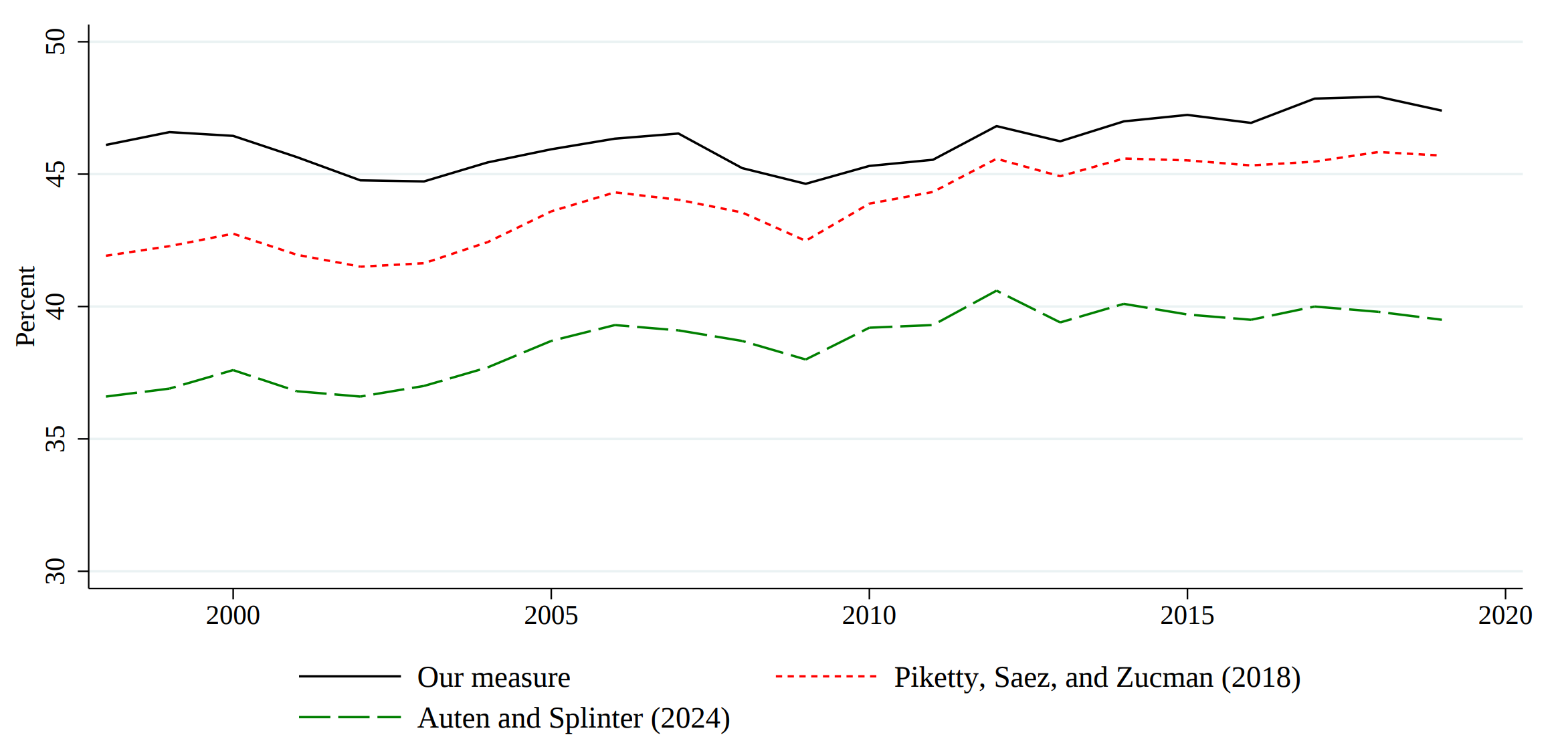
Figure 1 offers a glimpse at the suitability of our data for gauging trends in U.S. income inequality. The black line shows the share of gross income that accrues to the top 10 percent of the 18,836 zip codes that can be merged to the universe of 925 CBSAs. For comparison, the red dotted and green dashed lines show the share of gross U.S. income going to the top 10 percent of households nationwide, as estimated by Piketty et al. (2018) and Auten and Splinter (2024), respectively, using administrative tax records. Despite some level differences, our series tracks closely with these two widely used measures of income inequality over the 1998–2019 period and exhibits similar higher frequency fluctuations.

Figure 1. Top 10 Percent Income Share in the United States, 1998–2019

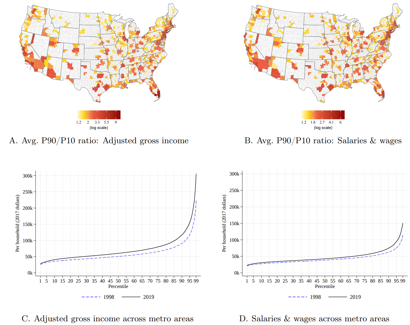
Panels A and B of Figure 2 illustrate the geographic dispersion of income inequality in our data – averaged over the 1998–2019 period – with inequality measured as the ratio of income per household in zip codes that are in the 90th percentile (P90) relative to income per household in zip codes that are in the 10th percentile (P10) of their respective CBSA distributions.³ Panels C and D, on the other hand, show the distributions of total income and labor income at the beginning and end of the sample period.⁴

Figure 2. Income Distribution across U.S. Metro Areas and Time

Three salient facts emerge from Figure 2. First, as shown in Panels A and B, both total and labor income are unevenly distributed across metro areas, with noticeably greater inequality observed in coastal areas. Second, some metro areas that are unequal with respect to the distribution of total income are also unequal in terms of labor income.⁵ Third, the distribution has become more unequal for both measures of income over the sample period, with both distributions becoming notably more skewed toward higher income levels in recent years.

Other Data

To understand the dynamic effects of monetary policy on the income distribution, we compute monetary policy surprises using changes in federal funds futures in narrow windows bracketing Federal Open Market Committee (FOMC) announcements, following the methodology developed by Miranda-Agrippino and Ricco (2021).

These policy surprises represent unanticipated shifts to the overall monetary policy stance, including the target range and the expected path of the federal funds rate, that are orthogonal to the state of the economy. The use of high-frequency monetary policy surprises ensures that the dynamic response of the income distribution that we estimate reflects unanticipated changes in the monetary policy stance and not other economic or financial developments to which policymakers may be responding. As our income data are available at only an annual frequency, we compute annual monetary policy surprises by summing the FOMC meeting-specific policy surprises for each calendar year in the 1998-2019 sample period.

Because U.S. metro areas differ significantly with respect to labor market conditions, industry structure, population dynamics, and sociodemographic characteristics like workforce education and race, we also use the available CBSA-level data from multiple sources to account for various confounding local factors. Our statistical analysis also controls for aggregate economic conditions that affect the entire cross section of CBSAs, such as inflation, output growth, the state of the national labor market, and broad financial conditions. After imposing some data filters and merging the CBSA-level income distribution data with data on local economic conditions, we are left with a slightly unbalanced panel of 317 CBSAs-all of which are MSAs-over the 1998-2019 period.

Dynamic Response of the Income Distribution to Monetary Policy

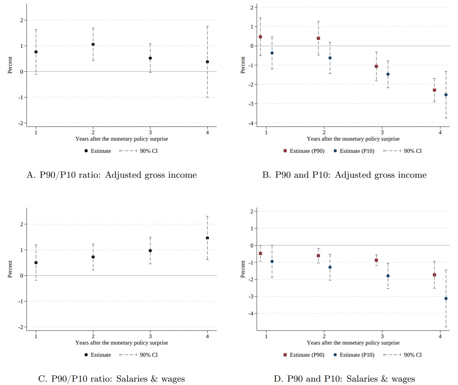
We estimate the dynamic response of the income distribution to monetary policy surprises using a panel version of the local projections framework proposed by Jordá (2005). Figure 3 shows the impulse responses of the within-MSA income distribution to an unanticipated tightening of monetary policy. The dots depict the point estimates of the impact of an unexpected monetary policy tightening of 25 basis points during year $t$ on the income distribution (in percent) in year $t+h$. The whiskers represent the 90 percent confidence intervals.⁶

Figure 3. Response of Income Inequality to a Monetary Policy Tightening

Panels A and C focus on total income inequality and labor income inequality, respectively, where inequality is measured as the logarithm of the P90/P10 ratio of the specified income variable. Panels B and D decompose these effects into separate responses at the 90th (P90) percentile and the 10th (P10) percentile of the distribution of the logarithm of (real) total income and the logarithm of (real) salaries and wages, respectively.

According to Panel A, following an unexpected 25 basis point tightening of monetary policy in year $t$, total income inequality is estimated to increase gradually over the subsequent two years, with the peak response of slightly more than 1 percent in year $t+2$. Thereafter, the effect of a policy tightening starts to weaken and by year $t+4$ is no longer statistically different from zero.⁷

Panel B shows that the increase in the P90/P10 ratio of total income in the first two years reflects both a rise in (real) income at the top decile (P90) of the income distribution and a decline in (real) income at the bottom decile (P10) of the income distribution. Thereafter, total income at the top and the bottom of the distribution both decline significantly and by roughly an equal amount, implying essentially no impact on the corresponding P90/P10 ratio.

Although movements in non-labor income may explain these differential responses, the absence of consistent reporting of financial and business income in our data prevents us from estimating the effects of monetary policy on each component of total income separately. Accordingly, the rest of our analysis relies on the comprehensive coverage of salaries and wages to analyze whether the distributional effects of monetary policy operate mostly though changes in the distribution of labor income.

Panel C provides evidence supporting the view that the labor market plays a key role in shaping the distributional footprint of monetary policy. Our estimates indicate that an unexpected 25 basis point cumulative tightening of monetary policy in year $t$ (roughly 1.5 standard deviations) leads to a cumulative rise in the average P90/P10 ratio of salaries and wages of about 3 percent – from 1.8 to 1.85 or about one within-MSA standard deviation – over the subsequent four years. This economically sizable effect is consistent with the view presented in the theoretical literature arguing that monetary policy primarily affects the dynamics of income inequality indirectly, namely through the heterogeneous exposure of labor income to changes in aggregate demand (see Kaplan et al., 2018; Auclert, 2019; Slacalek et al., 2020).

Given that the labor income distribution appears to be relatively more sensitive to changes in the monetary policy stance, a natural follow-up question is whether the distribution of wages and salaries widens because the lower part of the distribution responds to monetary policy more than the upper part. This question is also motivated by a finding that earnings of low-income workers fluctuate sharply with business cycles (see Heathcote et al., 2020; Bergman et al., 2022).

Panel D provides evidence that the distribution of wages and salaries widens because the lower part of the distribution responds to monetary policy more than the upper part. According to our estimates, starting in year $t+2$, the declines in (real) income accruing to the 10th percentile of the labor income distribution become, in absolute terms, notably greater than the corresponding declines in (real) income accruing to the 90th percentile. This divergence is consistent with the monotonically increasing impact of monetary policy on the P90/P10 ratio of labor income over the response horizon shown in Panel C.

The Role of Local Markets

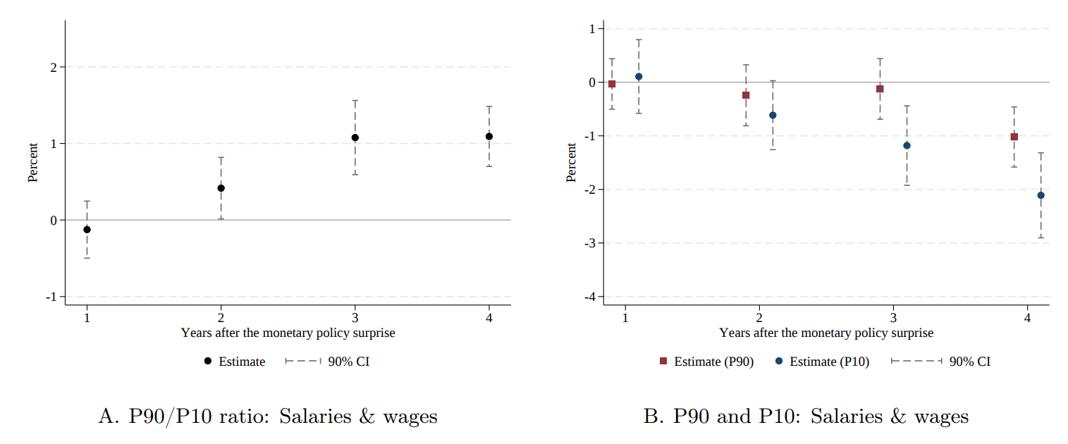
One possible explanation for the pronounced reaction of the bottom part of the labor income distribution to changes in the monetary policy stance is that the labor market outcomes of low-income workers are cyclically more sensitive to such changes compared with the outcomes of higher-income workers. To evaluate the strength of this explanation, Figure 4 reports estimates of the "excess" sensitivity of the labor income distribution to unanticipated tightenings in the monetary policy stance when local labor market conditions are weak – that is, when the local (MSA-specific) unemployment gap is positive and the local unemployment rate is above the national unemployment rate.

Figure 4. Response of Labor Income Inequality to a Monetary Policy Tightening (In Weak Local Labor Markets)

Figure 4 Panel A illustrates that beyond year $t+1$, weak local labor market conditions significantly amplify the policy-induced increase in earnings inequality. According to the point estimates, the P90/P10 ratio of salaries and wages increases by an additional 0.5 percentage points in year $t+2$ and by another full percentage point in both years $t+3$ and $t+4$, relative to the baseline effect shown in Panel C of Figure 3. These effects are economically large and statistically different from zero at the 10 percent significance level.

Furthermore, as shown in Panel B, the excess sensitivity of the response of the earnings distribution in weak local labor markets is driven entirely by the movement at the bottom of the labor income distribution. While an unanticipated tightening of policy leads to an economically sizable and durable decline in (real) salaries and wages at the bottom of the distribution, wages and salaries accruing to the top decile show no such excess sensitivity for most of the response horizon.

This evidence points to a pronounced heterogeneity in the response of income inequality to monetary policy across metro areas experiencing different labor market conditions. It also confirms that, for the most part, the distributional impact of monetary policy works through labor market outcomes of workers at the bottom of the income distribution, and especially so when local labor markets are already weak. These findings are consistent with previous research showing that unemployment rates, participation rates, and earnings of workers at the bottom of the income distribution are relatively more sensitive to aggregate demand and labor market cycles (see Aaronson et al., 2019).

References

Auclert, A. (2019): "Monetary Policy and the Redistribution Channel," American Economic Review, 109, 2333–2367.

Auten, G. and D. Splinter (2024): "Income Inequality in the United States: Using Tax Data to Measure Long-Term Trends," Journal of Political Economy, 132, 2179–2227.

Bergman, N., D. A. Matsa, and M. Weber (2022): "Inclusive Monetary Policy: How Tight Labor Markets Facilitate Broad-Based Employment Growth," NBER Working Paper No. 29651.

Bernanke, B. S. (2015): "Monetary Policy and Inequality," Commentary, The Hutchins Center on Fiscal and Monetary Policy. The Brookings Institution. Available at https://www.brookings.edu/blog/ben-bernanke/2015/06/01/monetary-policy-and-inequality/.

BIS (2021): "The Distributional Footprint of Monetary Policy," Bank for International Settlements, Annual Economic Report (Chapter II). Available at https://www.bis.org/publ/arpdf/ar2021e2.htm.

Draghi, M. (2016): "Stability, Equity, and Monetary Policy," 2nd DIW Europe Lecture, German Institute for Economic Research (DIW), Berlin, October 25, 2016. Available at https://www.ecb.europa.eu/press/key/date/2016/html/sp161025.en.html.

Heathcote, J., F. Perri, and G. L. Violante (2020): "The Rise of US Earnings Inequality: Does the Cycle Drive the Trend?" Review of Economic Dynamics, 37, 181–204.

Jordà, Ò. (2005): "Estimation and Inference of Impulse Responses by Local Projections," American Economic Review, 95, 161–182.

Kaplan, G., B. Moll, and G. Gianluca L. Violante (2018): "Monetary Policy According to HANK," American Economic Review, 108, 697–743.

Miranda-Agrippino, S. and G. Ricco (2021): "The Transmission of Monetary Policy Shocks," American Economic Journal: Macroeconomics, 13, 74–107.

Piketty, T., E. Saez, and G. Zucman (2018): "Distributional National Accounts: Methods and Estimates for the United States," Quarterly Journal of Economics, 133, 553–609.

Slacalek, J., O. Tristani, and G. L. Violante (2020): "Household Balance Sheet Channels of Monetary Policy: A Back of the Envelope Calculation for the Euro Area," Journal of Economic Dynamics and Control, 115, 1038–1079.