Board of Governors of the Federal Reserve System

December 07, 2018

Overview of the changes to the FRB/US model (2018)

Introduction

The FRB/US model was launched almost 25 years ago as a large macroeconomic model of the US economy. References and documentation about the FRB/US model and some of its history can be found on the public website.¹ While the model has been modestly updated and changed over the years, this FEDS Note summarizes a more comprehensive set of modifications introduced with the November 2018 public release of the model and provides some motivation for why they were made.

Many of the modifications in this release aim to reduce the complexity and scope of the model via the consolidation, aggregation or elimination of various model variables and equations whose contribution to the major properties and uses of FRB/US is relatively minor. In light of the costs inherent to the operation and maintenance of a large and complex model like FRB/US, these simplifications reflect our judgement that a benefit-cost analysis suggests a somewhat smaller model. Other modifications deal with improvements in selected model properties such as the tempering of near unit root dynamics in response to certain shocks.

Although the size of the model has been reduced from more than 500 variables to about 370 variables, by design these changes do not substantially alter the model's dynamics, especially in the short-to-medium run. These modifications provide a foundation from which future efforts to improve the core of the FRB/US model can proceed, taking into account various developments that have occurred in the field of macroeconomics over the past 25 years, while at the same time maintaining the overall philosophy that has characterized the model since its inception.

Bird's Eye View of the Changes to the FRB/US Model

The changes to the FRB/US model can be organized in six categories.

1. Simplification of potential output and elimination of energy as a factor of production

Energy has been dropped as a factor of production. Although the model will no longer be able to quantify the effects on potential output of changes in the relative price of energy, the benefits of this capability have always been minor if not negligible. For example, the contribution of historical energy price movements to the model's estimate of the four-quarter growth of potential output has rarely exceeded a tenth of a percentage point. On the other side of the ledger, substantial modeling costs have been eliminated.

Many of these costs come from the need to associate production with a concept of business output that is adjusted (XG) to include oil imports. Not only did the existence of this non-standard measure of output create maintenance and pedagogical burdens, it also placed a priority on being able to adequately model oil imports, so that the production function's measure of potential output was accurately translated into domestic potential. But modeling oil imports has become more complicated in the past decade, as the price-sensitivity of domestic production has risen. This development had made the model's exogenous treatment of domestic energy production inadequate. If the energy factor were retained, the FRB/US model would need to expand its energy sector to contain an endogenous specification of energy production. Another issue associated with the translation of adjusted output to the NIPA measure of business output was that it involves chain weighted aggregation, which as discussed below, generates non-stationarities in the model's dynamics.

We also simplified some other parts of the energy sector, including how oil imports are modeled. Previously, the price and quantity of domestic energy consumption were the key endogenous drivers of oil imports, which were determined by the difference between domestic energy consumption and (exogenous) production. In the new version of the model, the ratio of oil imports to GDP is a simple reduced-form function of a stochastic trend and the relative price of oil imports. This change permits the price and quantity of domestic energy consumption and the quantity of domestic energy production to be removed.

2. Aggregation of business fixed investment

We simplified the business (i.e. nonresidential) investment sector by modeling business fixed investment as a whole rather than three separate components (equipment, intellectual property and software, and structures). Our experience over the past decade indicates that the presence of disaggregated components of investment has never been crucial, while the costs of maintaining the disaggregation have been a noticeable burden. Simulations show that the behavior of aggregate investment (and the rest of the economy) is similar whether investment is modeled at a disaggregated level or not. The same general specification that was previously applied to each component of business investment is applied to their aggregate.

3. Simplification of the government sector

We have consolidated many components of the fiscal sector, both across the federal and state and local (S&L) levels of government and, where separate federal and S&L variables remain, within each level. The simplified version preserves key federal variables (e.g. debt and surplus). To the extent that these key federal variables are now specified as functions of the newly created consolidated fiscal variables, their equations include adjustment factors to isolate the federal contribution. The only area where the federal and S&L distinction is preserved is (gross) government expenditures. Here, the distinction is also important to accurately model the remaining federal variables. Some simplifications of the expenditure side of the government sector are nonetheless possible, as the disaggregation of (gross) expenditures at each level of government can be reduced from three to two components.

4. Replacement of all chain aggregation formulas by linear approximations with fixed weights

Following the approach used in the National Accounts for constructing historical measures of quantity aggregates, FRB/US has long used some forms of chain aggregation for constructing simulated values of such aggregates. Recently, however, we have identified the non-linear nature of the chain aggregation formulas (or their near equivalents) as one of the main reasons behind artificial asymmetries in the response of key economic variables to the model's shocks. Such asymmetries are one consequence of the path dependent dynamics that these types of formulas create in a model like FRB/US. Path dependence also adds extra unit roots to the model, which in turn cause many types of transitory shocks to have unwarranted (albeit small) long-run macroeconomic effects. The new version of the model moves to a formulation for aggregation (log-linear with time-invariant weights) that does not generate these types of spurious behavior. The benefits from this shift exceed any costs associated with the introduction of approximation errors by the use of fixed weights for aggregation.²

5. Elimination of the compounded annualized rate series

The previous version of FRB/US contained two concepts of most interest rates: the effective annualized yield and the stated interest rate. The former accounts for compounding over the full year and this concept was assumed to govern the behavior of agents in the model. The latter concept corresponds to the way market interest rates are quoted in practice. In this release, effective interest rates have been eliminated from the model and quoted rates are assumed to govern behavior. With the low interest rates prevailing under current circumstances, the quantitative differences between the concepts is relatively small, the elimination of one of them appeared to be a natural course of action.

6. Other miscellaneous simplifications and improvements

The new version contains some other modifications to parts of FRB/US whose contributions are marginal. The most salient changes in this category are:

• The simplification of the block associated with the consumption of fixed capital (CFC).
  • Many minor variables capturing the contribution of the government CFC have been dropped.
  • The equation for CFC in the private sector is simplified.
• Some minor household income variables (property and rent related) are consolidated.
• Variables that have very close counterparts in the model have been eliminated. Examples of such variables include a second set of aggregate measures of the exchange rate and foreign prices that differ only by the bundle of countries use to calculate the weights.
• The modifications to the variables and equations for CFC and household income aim to improve the long-run dynamics (i.e. 10 years or later) of FRB/US. These aspects of the model have been shown in some simulations to lead to undesirable features in the long-term while the modifications show no apparent effects on the short-run properties.

Effects of the revisions on the dynamic responses to key shocks

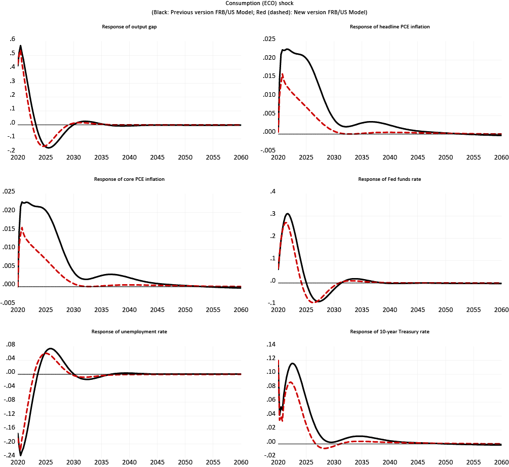
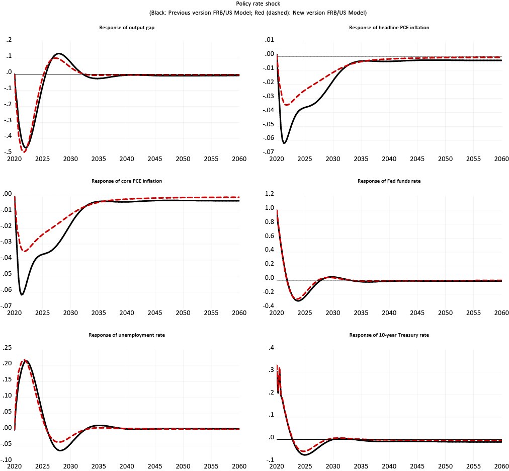
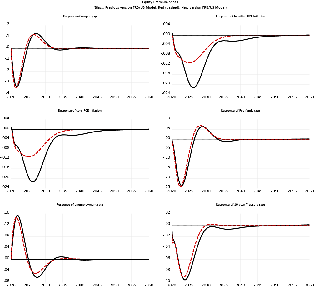
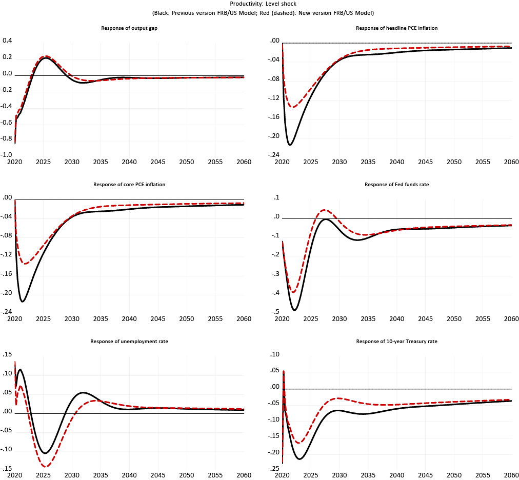
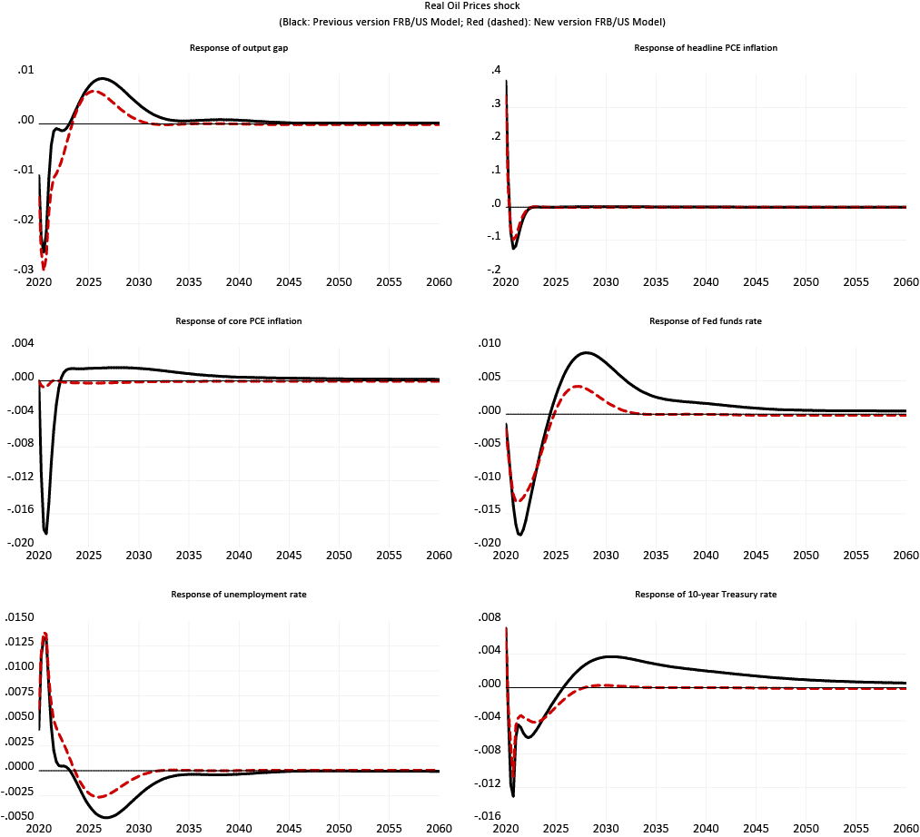
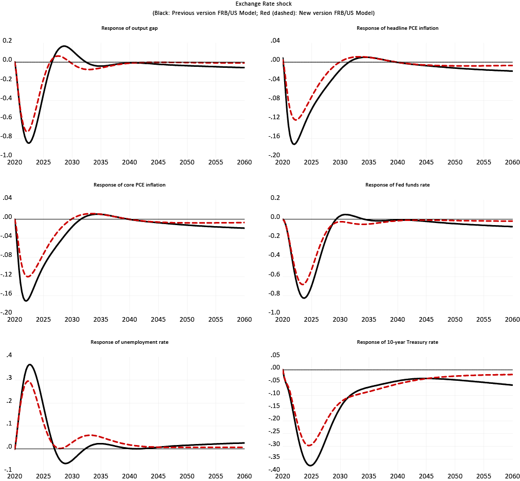
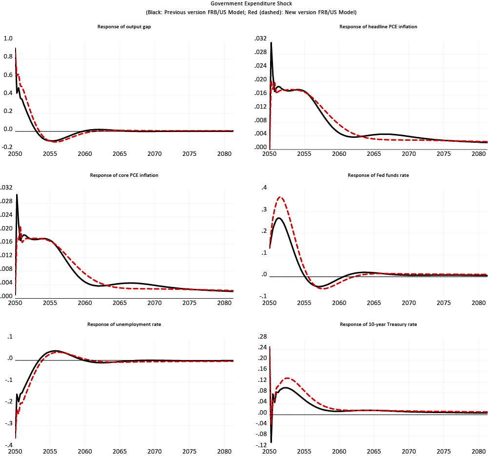
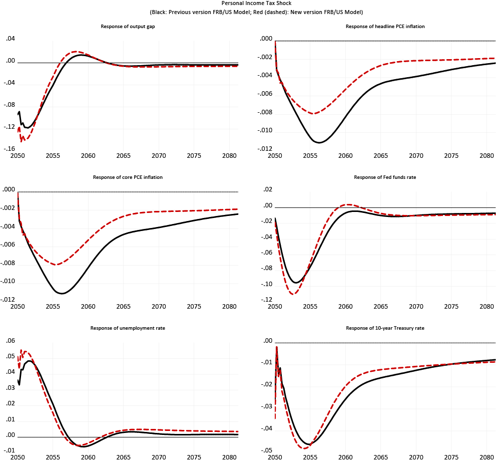
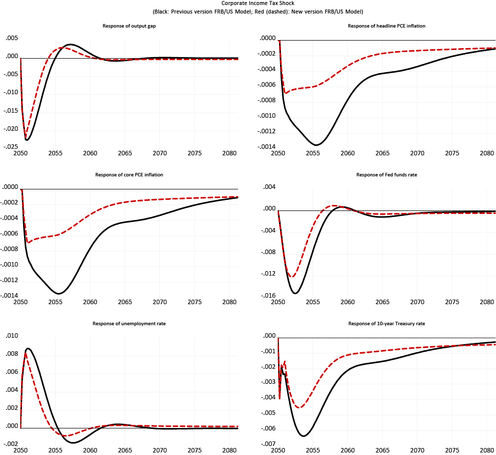
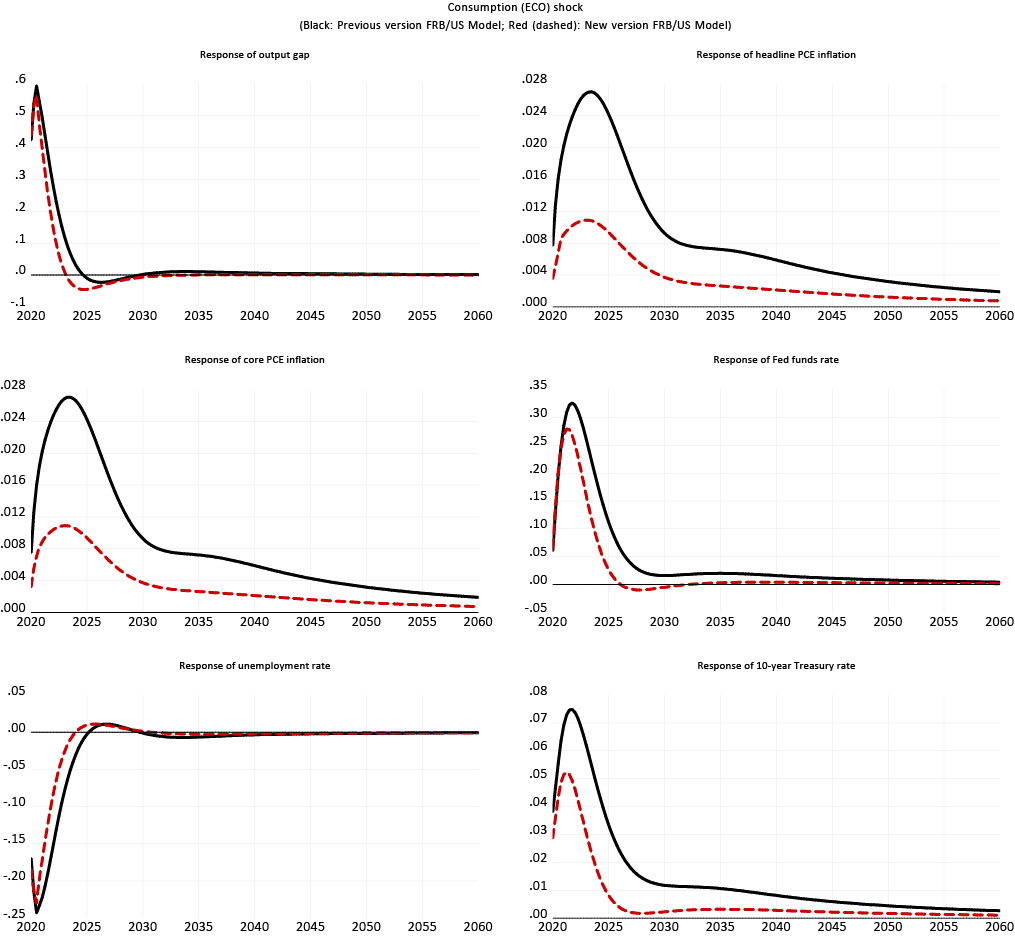
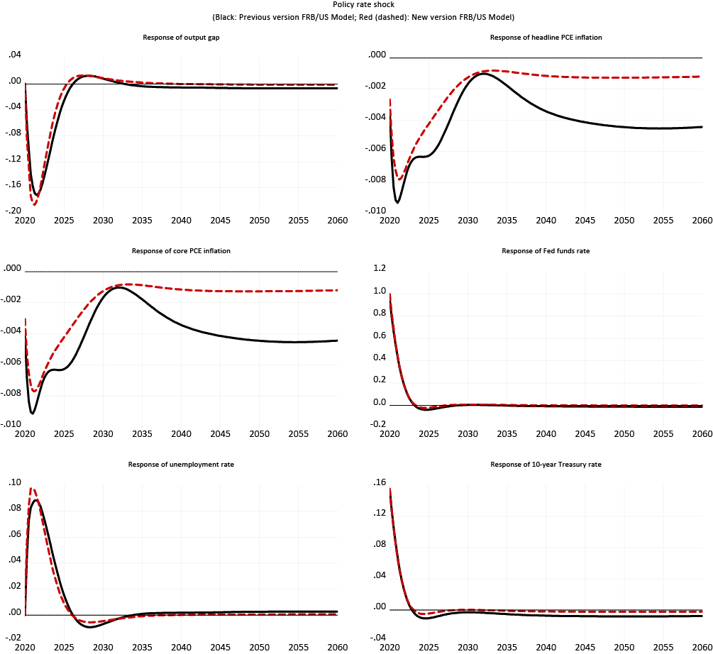
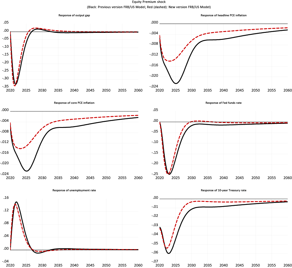
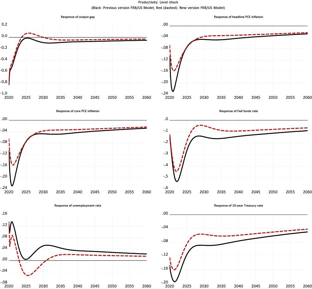
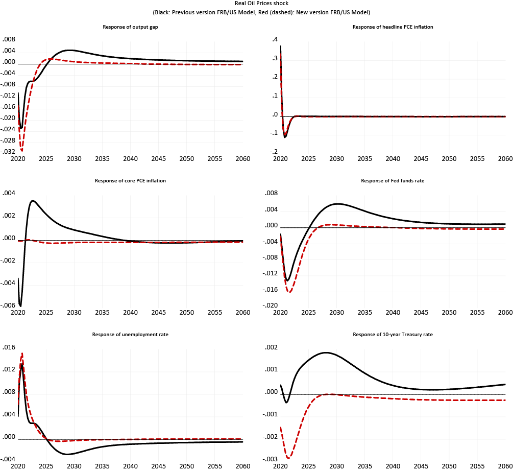
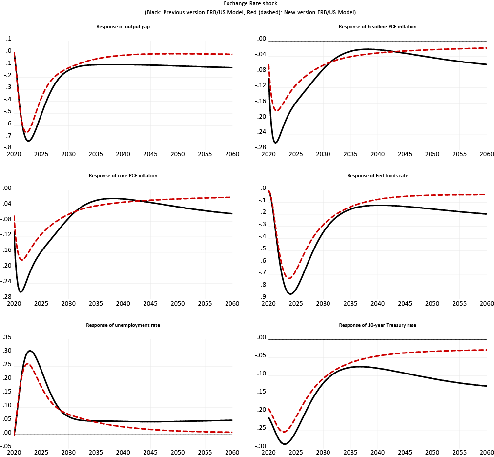
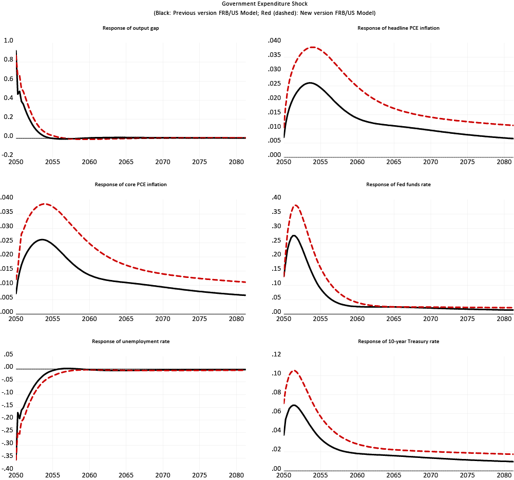
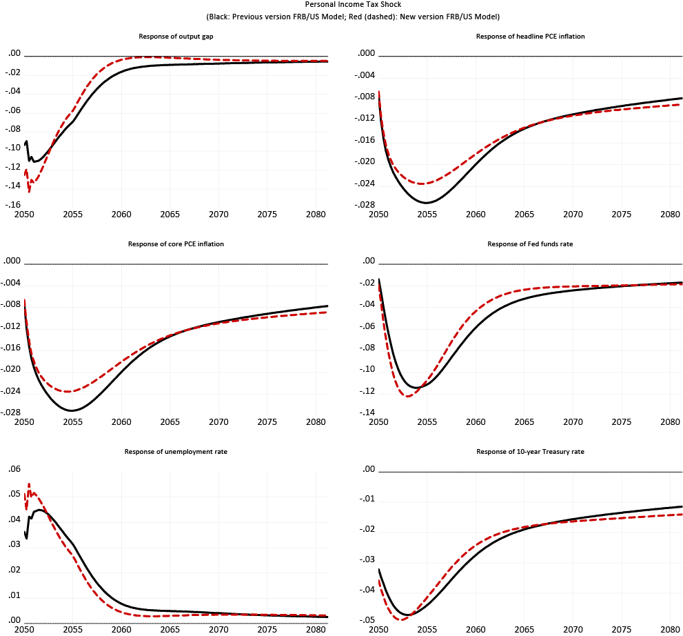
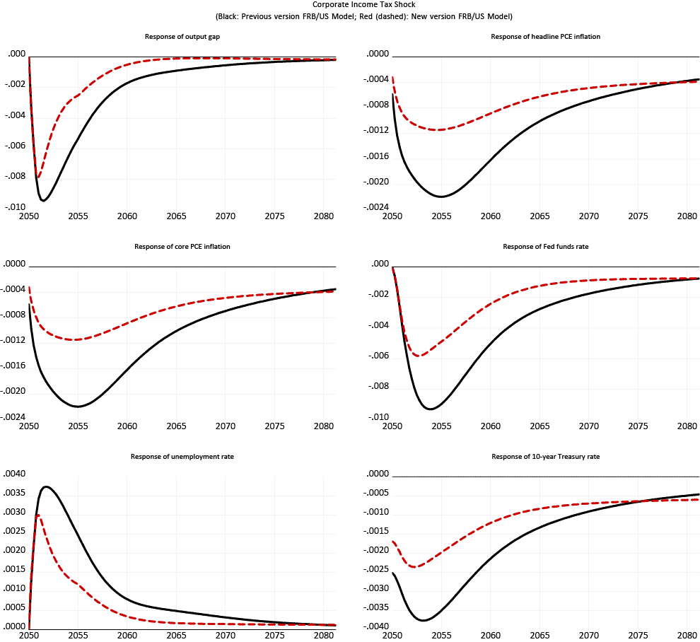
This section presents and discusses very briefly the impact of the changes to FRB/US on its dynamic responses to nine shocks: consumption demand, monetary policy, equity premium, productivity, oil price, exchange rate, government expenditures, and personal income and corporate income average tax rate shocks. We show the responses under two expectation settings: VAR-based (figures 1-9) and model-consistent expectations (figures 10-18).³ In all the simulations, the dynamics follow from a one-time shock to the equation of interest. As noted in the introduction, the objective of the changes to the FRB/US was to simplify the structure of the model without introducing major changes (unless desired) to the model dynamic properties. The figures show simulation results that are broadly consistent with this statement. The responses of the output gap, unemployment rate, fed funds rate and long-term interest rate are very similar across the two versions of the model. Although the sensitivity of the inflation process has declined in the new model, the smaller short-term responses of the inflation variables reflect not so much the changes to the model as they do the re-estimation of the wage-price block equations over a longer sample period that now extends through 2017. An update of the estimation of the old version of the FRB/US would have resulted in smaller responses of the inflation process as well. A second noticeable feature of the responses between the models is a faster convergence of the response of many variables back to the original baseline in the long run.

Figure 1: Responses to a 1 percent increase in consumption (ECO) (VAR-based expectations)

Figure 2: Responses to a 100 bps increase in the Fed funds rate (VAR-based expectations)

Figure 3: Responses to a 100 bps increase in the equity premium (VAR-based expectations)

Figure 4: Responses to a 1 percent in the level of productivity (MFPT) (VAR-based expectations)

Figure 5: Responses to a 10 dollar increase in oil prices (VAR-based expectations)

Figure 6: Responses to a 10 percent increase the real exchange rate (through FPXRR) (VAR-based expectations)

Figure 7: Responses to a one-time increase in government expenditures by 1 percent of GDP (VAR-based expectations)

Figure 8: Responses to a one-time 1 percentage point increase in the average personal income tax rate (VAR-based expectations)

Figure 9: Responses to a one-time 1 percentage point increase in the average corporate income tax rate (VAR-based expectations)

Figure 10: Responses to a 1 percent increase in consumption (ECO) (Model-consistent expectations)

Figure 11: Responses to a 100 bps increase in the Fed funds rate (Model-consistent expectations)

Figure 12: Responses to a 100 bps increase in the equity premium (Model-consistent expectations)

Figure 13: Responses to a 1 percent in the level of productivity (MFPT) (Model-consistent expectations)

Figure 14: Responses to a 10 dollar increase in oil prices (Model-consistent expectations)

Figure 15: Responses to a 10 percent increase the real exchange rate (through FPXRR) (Model-consistent expectations)

Figure 16: Responses to temporary increase in government expenditures by 1 percent of GDP (Model-consistent expectations)

Figure 17: Responses to a temporary 1 percentage point increase in the average personal income tax rate (Model-consistent expectations)

Figure 18: Responses to a temporary 1 percentage point increase in the average corporate income tax rate (Model-consistent expectations)