FEDS Notes
October 22, 2021
Wealth Inequality and the Racial Wealth Gap
Aditya Aladangady, and Akila Forde
In the United States, the average Black and Hispanic or Latino households earn about half as much as the average White household and own only about 15 to 20 percent as much net wealth. As we see in Figure 1 below, this wealth gap has widened notably over the past few decades (left panel).1 At the same time, overall wealth inequality—as measured by the Gini in the right panel—has also grown. In this Note, we introduce a novel method to decompose measures of inequality. Our decomposition allows us to compare actual wealth inequality with a counterfactual world without racial wealth gaps, but where inequality overall remains as in the data. The decomposition allows us to quantitatively answer a number of questions: How do differences in racial composition at various points in the wealth distribution contribute to overall inequality? How have these differences evolved over time, and how do widening racial wealth gaps contribute to rising inequality? And how have differences across racial and ethnic groups in portfolio composition and returns affected inequality?
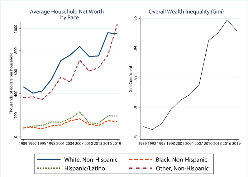
Source: Survey of Consumer Finances.
A racial equality counterfactual
In order to quantify how far our world is from racial equality—and how this wedge has evolved in recent history—we need to first define what "racial equality" means. In this note, we adopt a specific racial equality counterfactual which assumes households of all races are equally represented at all points in the wealth distribution in proportion to their population shares. That is, households in the bottom 10 percent of the wealth distribution have exactly the same racial composition as those in the top 10 percent or any other point in the distribution. This situation represents one where there is no inequality between races, but overall wealth inequality remains as it is in the US.
One way to view this counterfactual is through the lens of a Oaxaca-Blinder or similar decomposition that allows us to separate between-group and within-group inequality. The racial equality counterfactual we consider reduces between-race inequality to zero and raises within-race inequality for each race in order to keep overall inequality as it is in the data. By doing so, our counterfactual world can somewhat abstract from concerns about how changes in the wealth distribution may impact aggregate savings, interest rates, or other macroeconomic outcomes.2
Reality differs considerably from this counterfactual. Looking at the population as a whole, White households hold 86.8 percent of overall wealth in the country according to the 2019 SCF, though they account for only 68.1 percent of the households in the survey.3 By comparison, Black and Hispanic households hold only 2.9 and 2.8 percent of wealth, respectively, while accounting for 15.6 percent and 10.9 percent of the US population respectively, reflecting the fact that wealth is disproportionately skewed towards White households. In fact, under racial equality, Black households would hold over 5 times the amount of wealth they currently do, and Hispanic households would hold nearly 4 times as much.
A shift to the racial equality counterfactual would affect households at various points in the wealth distribution differently. Table 1 shows how the average net worth of households of each race would change for each quartile of the wealth distribution. The average Black household in the top quartile of wealth would have over twice the amount of wealth under the racial equality counterfactual than they do currently, and the average Hispanic household in the top quartile would see an 86 percent increase. Meanwhile, White households in the top quartile would give up around 5 percent of their wealth.4
Table 1: Change in Average Household Net Worth by Moving to Racial Equality Counterfactual
| Wealth Quartile | ||||
|---|---|---|---|---|
| Bottom | Bottom-Middle | Top-Middle | Top | |
| White, non-Hispanic | -13% | -5% | -1% | -5% |
| Black, non-Hispanic | 22% | 9% | 3% | 117% |
| Hispanic | 92% | 10% | 6% | 86% |
| Other | -51% | 17% | -6% | -1% |
At the other end of the distribution, Hispanic households—who constitute a large share of very low wealth households—would see a 92 percent increase in wealth from shifting to racial equality, and the average Black household in the bottom quartile would see a 22 percent increase. Notably, a shift to racial equality without changing overall inequality hurts low-wealth White households, who would see a 13 percent decline in wealth.
The middle of the distribution—particularly around the third quartile—appears quite close to racial equality currently, and a shift to the racial equality counterfactual would result in relatively small changes in wealth for the average households at this point in the distribution.5 Overall, the results suggest racial inequities are concentrated at the extremes of the distribution, with White households disproportionately accounting for very high wealth segments and Black and Hispanic households disproportionately accounting for lower wealth segments.
Quantifying racial wealth gaps using a Gini decomposition
Given the racial equality counterfactual we laid out, we need a metric to quantify how far the actual wealth distribution is from the counterfactual, and how this gap has evolved over time. In order to quantify how far we are from racial equality, we introduce a new decomposition of the Gini coefficient—a standard metric of inequality—that allows us to summarize the distance we are from racial equality and how various groups are contributing to this gap. In particular, the decomposition allows us to quantify how the Gini would change if each racial group held wealth in a distribution similar to the aggregate wealth distribution.
The Gini coefficient is based on the Lorenz curve for household wealth, a function that tells us the fraction of overall wealth in the country owned by the bottom x percent of the population for various values of x. Figure 2 plots the Lorenz curve for net worth using the 2019 wave of the SCF. Under perfect equality, the curve would lie precisely on the 45-degree diagonal (the dashed line), such that the bottom 50 percent of households ranked by wealth would hold 50 percent of overall wealth, etc. Instead, the curve is significantly bowed down, such that the bottom 50 percent of households own just 1.5 percent of overall household wealth.6
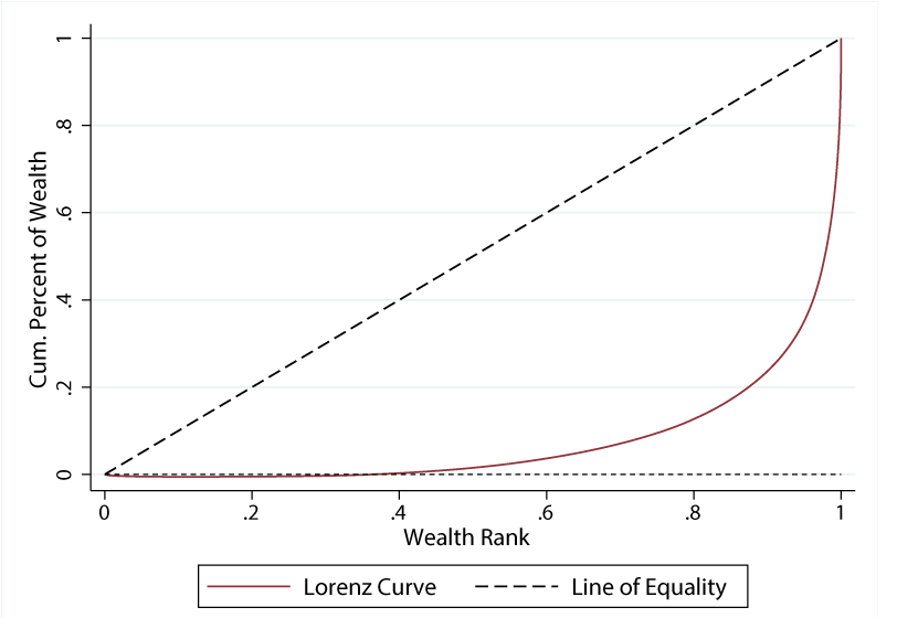
Source: Survey of Consumer Finances, 2019.
The Lorenz curve also provides a means to decompose wealth across types of households, such as households of different races. The top-left panel of Figure 3 takes the same Lorenz curve as in Figure 2 (the solid black line just above the shaded regions) and splits it into the fraction of wealth held by White/non-Hispanic households (blue), Black/non-Hispanic households (yellow), Hispanic/Latino households (green), and households of other races (red). The figure shows that White households (the blue region) accounts for a high share of the area under the curve—in fact, more than their population share, as mentioned previously. This is consistent with the fact that minority households are concentrated toward the bottom of the wealth distribution, whereas White households are concentrated at high wealth levels, as shown in the bottom-left panel which shows population shares by race at each wealth quantile.
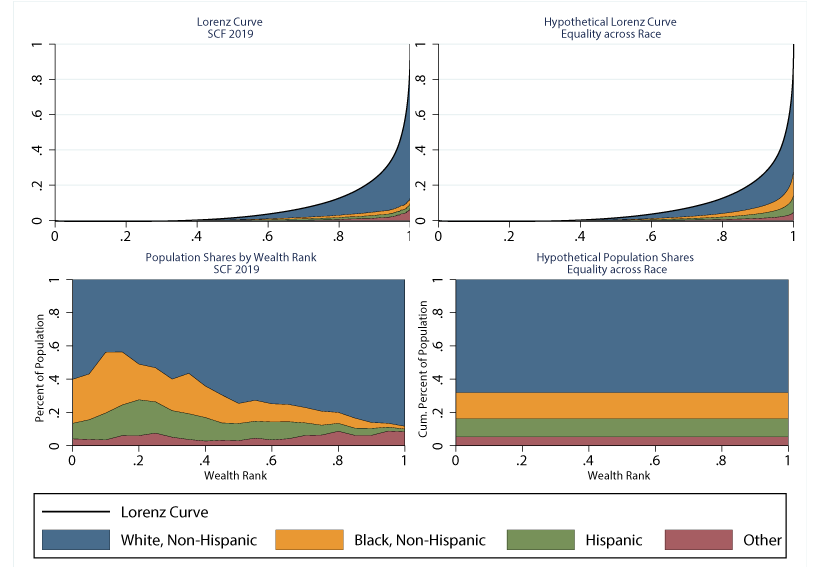
Note: Shaded regions appear in order of legend from top to bottom. Source: Authors' calculations using Survey of Consumer Finances.
The right panels show how this same decomposition looks in the "racial equality" counterfactual. Given our definition of racial equality, we see in the bottom-right panel that the racial composition does not vary across the wealth distribution, and the top-right shows the overall Lorenz curve remains the same, since the wealth distribution is unaltered. However, the decomposition is shifted such that White households hold much less wealth (i.e., the overall blue region is smaller) and minorities hold more wealth in the upper parts of the wealth distribution (i.e., the other regions are more concentrated toward higher wealth levels).
The Lorenz curves in Figure 3 provide a detailed view into the racial composition of wealth holdings across the distribution, similar to what we saw in Table 1. In addition, the Lorenz curve allows us to summarize the decomposition using a standard metric of inequality, the Gini coefficient. In particular, the Gini coefficient is given by $$G=1-2*A$$ where $$A$$ is the area under the Lorenz Curve (all the colored regions in the top-left of Figure 3). Higher values of the Gini suggest the Lorenz Curve is further from the line of equality, and overall wealth inequality is higher. Since the actual and counterfactual Lorenz Curves are identical, their overall Gini coefficients are both the same (0.852 in 2019). However, the composition of the area A differs between the two, based on how much households of each race are under- or over-represented at each quantile of wealth and what share of overall wealth is held by that quantile. The difference between the composition in each panel can provide a measure of how much households of each race are contributing to overall inequality relative to the racial equality counterfactual, as summarized by the Gini.7 In particular, the difference in each colored region (for each race) tells us how overall inequality would change if the wealth among households of each race were distributed the same as the aggregate wealth distribution—as in the racial equality counterfactual—instead of how it is in the actual data.
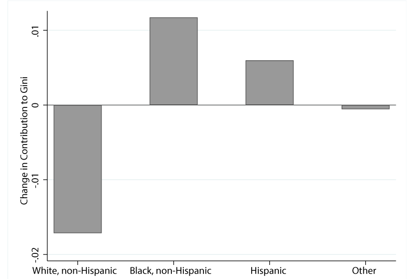
Note: Bars denote difference in Gini contribution for each race in racial equality counterfactual versus actual SCF data in 2019 and are derived by differencing the shaded regions in the top panels of Figure 3. Each bar represents the change in Gini achieved by shifting the distribution of each race's wealth to match the aggregate wealth distribution. Contributions sum to zero by assumption. Source: Authors' calculations using Survey of Consumer Finances.
Figure 4 above provides this decomposition. Shifting the wealth of White households to match the overall wealth distribution—as in the racial equality counterfactual—would lower the Gini by 1.7 points, or about a quarter of the increase in inequality seen over the past three decades. Doing the same for Black and Hispanic households would raise inequality by 1.2 and 0.6 index points since these groups hold much less wealth than the average American. Households of other races are more evenly represented across the distribution on average, as reflected by the small change relative to racial equality. However, this result likely masks considerable heterogeneity between subpopulations grouped into this category. Of course, on net, overall inequality would be unchanged by shifting to the racial equality counterfactual by assumption, and the bars for each racial group in Figure 4 sum to zero by construction.
It is a well-known fact that income inequality has been on the rise in recent decades, and wealth inequality has largely followed a similar pattern (Piketty & Saez, 2003; Saez & Zucman, 2016; Bricker et al, 2016). Indeed, we saw in Figure 1 that the Gini coefficient from the SCF data has risen from .787 in 1989 to .852 in 2019. We can use the decomposition above to also understand how racial disparities interplay with trends in inequality over time.
Figure 5 decomposes the change in the Gini coefficient since 1989 into contributions from each racial group. The Gini rises by exactly the same amount in both the true data (solid line, top-left) and the racial equality counterfactual (top-right), but the contributions of each racial group to the increase in inequality differs. Of course, the larger population share of White households leads them to contribute more to inequality growth even in the counterfactual, but the increase is driven disproportionately by this group in the true data. To make the differences between the panels more clear, the bottom panel shows how much extra each race contributes to inequality growth compared to the racial equality counterfactual.8 Since the overall Gini is the same, the bars add to zero, but growth in inequality is clearly driven disproportionately by White households.
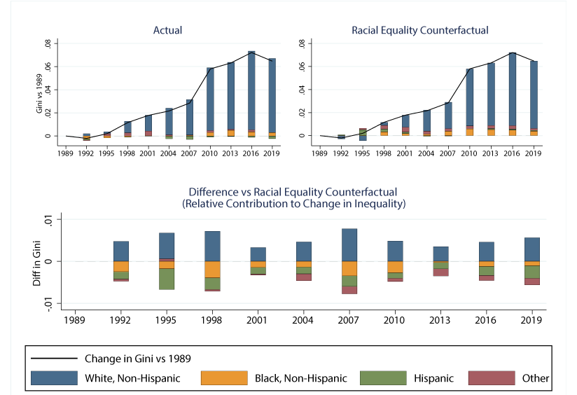
Note: Contributions to difference appear from top to bottom in order they appear in legend, except in 1992 and 1995 when "Other" appears just below "White." Source: Authors' calculations using Survey of Consumer Finances.
The result above pools all White households together, though we know from existing studies that inequality growth is driven in large part by the top tail of the distribution pulling further away from the rest (Piketty & Saez, 2003; Saez & Zucman, 2016; Bricker et al, 2016). As we have shown previously, this tail is largely comprised of White households. As these households pull away, they exacerbate racial wealth gaps, and also raise within-White inequality. As such, the blue bars above contribute an outsized amount to rising inequality. However, the truth is more complex than just that, as Suarez & Thompson (2019) point out. In their paper, they show that even conditional on many observable characteristics, minority households hold lower wealth than their White counterparts, particularly at the top of the wealth distribution. As such, some factors correlated with race are holding back minority households' ability to accumulate wealth and reach the top of the distribution at the same rates as Whites.
A number of possible factors may drive the growing wedge. One reason wealth disparities may persist is due to differences in initial wealth, income, and saving rates. As we have seen in Figure 1, a long history of discrimination has left Black and Hispanic households with substantially less wealth even in the beginning of our sample period. Moreover, Black and Hispanic households earn considerably less than White households, limiting their ability to save and build wealth.9 Indeed, Suarez & Thompson (2019) find that income differences do explain a part of the racial wealth gap, though a substantial gap exists even after conditional in earnings.10 Wealth gaps may also persist across generations as young minority households are less likely to receive intergenerational transfers from their parents. As Feiveson & Sabelhaus (2018) show, both intra-vivos transfers and end-of-life bequests are concentrated among higher-wealth and predominantly White households.
Another reason racial disparities in wealth may persist is due to differences in the types of assets households hold and the returns on these assets. In fact, portfolios look quite different across the wealth distribution, as shown in Figure 6 below. Households at the bottom hold very little wealth, often in the form of liquid financial assets—bearing relatively low levels of interest--countered by considerable debts. The physical assets they do have tend to be things like cars (captured in "Other net wealth"), which tend to depreciate in value quickly. As we go up the distribution, portfolio shares shift toward home equity, with business and financial wealth becoming a larger share towards the very top. Importantly, the asset classes held by high wealth households also generate positive returns through both interest income and capital gains. Notably, capital gains are taxed at lower rates than income, thereby providing a higher after-tax flows which can be further saved.
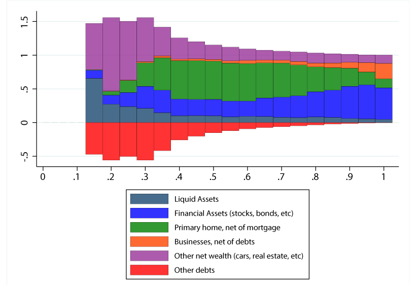
Note: Contributions appear from x-axis up in the order they appear in the legend, with exception of Other Debts, which appears below the x-axis. Portfolio shares for bottom quantiles with negative net wealth not plotted. Source: Survey of Consumer Finances, 2019.
In addition to differences in portfolio composition, returns within a specific asset class may differ across households (Fagereng, et al 2020). Quantifying the importance of these differences is difficult in our data, as we do not observe returns directly. Therefore, we focus on housing, which is both an important driver of inequality and also an asset for which we can observe returns based on local house price dynamics and leverage.11 Relative to other broad asset classes, heterogeneity in housing returns may also be less likely to reflect risk preferences or other factors that typically influence portfolio choice, and instead be driven by preferences for neighborhoods, access to labor markets in a given city, or housing supply limitations in the area.
In the chart below, we attempt to quantify average returns on housing and home equity for households of various races. To do this, we construct an average return on housing by weighting county-level house price growth by the distribution of households of a given race in those areas.12 Though our county-level analysis masks neighborhood-level heterogeneity in house prices within counties, it provides a bound on differences in housing returns across races.13
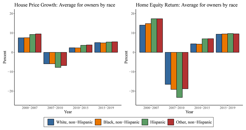
Note: Legend entries appear in the graph from left to right. Home ownership rates from 2000-2004 are from 2000 Census, 2005-2019 are from 1-year ACS in each year.
Source: Authors' calculations using 2000 Decennial Census, 2005-2019 American Community Survey, CoreLogic, Inc, HPI data, and Black Knight McDash.
In the left panel, we can see that the average Black and White homeowners saw their homes appreciate and depreciate by similar amounts, while Hispanic owners saw a bit more volatility in house price growth. However, the amount of leverage—the fraction of home value financed by a mortgage—can amplify the gain or loss in housing values as a percent of their net wealth in housing. Once we account for leverage, as we do in the right panel, it appears non-White households fared considerably worse in the financial crisis. In the five years after the financial crisis, returns were somewhat higher for the average Hispanic household than both Black and White households, but returns seem similar across groups since 2015 or so. While our evidence may be a lower bound on the heterogeneity in returns, it is consistent with recent evidence that minority households—whose neighborhoods are more prone to foreclosures and distressed sales—may suffer more volatility in returns and sharper declines during bad times (Kermani & Wong, 2021).
The fact that Black households have fared poorly in the wake of the financial crisis is likely exacerbated by the fact that the home ownership rate among Black households declined steadily from 2005 to 2015 and then bottomed out near its level in the mid-1990s. We see this in Figure 8, which indexes ownership rates by race to 1994 to highlight changes over time. (Ownership rates among White households have remained considerably higher than for minorities, with White home ownership at 73.7 percent at the end of 2019 compared to 44 percent for Black households and 48.1 percent for Hispanic households.) Notably, White and Hispanic households fared better over this period, with Hispanic households actually closing the ownership gap with White households some. Nonetheless, the lower homeownership levels suggest minority households, and Black households in particular, did not reap the benefits of rising home prices over recent years.
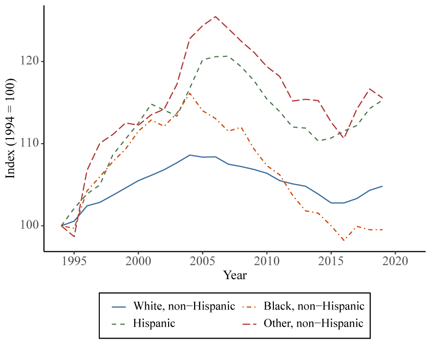
Source: U.S. Census, Housing Vacancies and Ownership.
Conclusion
Our results quantifying racial wealth gaps through the lens of a Lorenz curve decomposition and a racial equality counterfactual, complementing existing studies that document pre-existing wealth gaps across racial lines. In particular, our decomposition allows us to compare our world with a counterfactual where overall wealth inequality is the same as reality, but there are no differences in the distribution of wealth holdings across race. By doing so, we can isolate the impact of racial disparities relative to changes in overall inequality, which may impact other features of the economy in general equilibrium.
The decomposition allows us to highlight a few major facts. First, White households hold a much larger share of wealth than their population share, with Black and Hispanic households disproportionately concentrated at low, or even negative net wealth ranges. In fact, shifting the distribution of wealth among White households to match the aggregate distribution would lower inequality by 1/4 of its increase over the past three decades. Second, White households as a whole contribute more to both the level and growth in inequality than they would under a racial equality counterfactual. This reflects the fact that high-wealth households, who are predominantly White, have pulled away from the rest of the distribution over time. The divergence likely reflects a combination of ability to save, access to high-return assets, and other factors mean White households are, on average, more able to accrue and grow their wealth than minorities. One of the most prevalent means of accruing wealth for minority households, homeownership, has become less common among Black households in recent years, allowing the wealth gap to widen.
These pre-existing differences in wealth holdings across races may interact with how households are able to weather the strains brought about by the pandemic and subsequent recession. In particular, minority households are less likely to own assets to mitigate the impacts of job losses, or own homes or stocks which would allow them to gain from the unusually solid stock market and house price gains after the Great Recession. Differences across races in home ownership and leverage may also mean minority households disproportionately benefit from rent moratoriums and forbearance programs (An et al., 2021).
References
Altonji, Joseph; Ulrich Doraszelski and Lewis M. Segal, (2000), Black/white differences in wealth, Economic Perspectives, (Q I), 38-50
An, Xudong and Cordell, Larry and Geng, Liang and Lee, Keyoung, Inequality in the Time of COVID-19: Evidence from Mortgage Delinquency and Forbearance (February 20, 2021). Available at: http://dx.doi.org/10.2139/ssrn.3789349
Barsky, Robert, John Bound, Kerwin Kofi Charles and Joseph P. Lupton. "Accounting For The Black-White Wealth Gap: A Nonparametric Approach," Journal of the American Statistical Association, 2002, v97(459,Sep), 663-673.
Bhutta, Neil, Andrew C. Chang, Lisa J. Dettling, & Joanne W. Hsu, (2020). "Disparities in Wealth by Race and Ethnicity in the 2019 Survey of Consumer Finances," FEDS Notes 2020-09-28-2, Board of Governors of the Federal Reserve System (U.S.).
Blau, Francine and John W. Graham, (1990), Black-White Differences in Wealth and Asset Composition, The Quarterly Journal of Economics, 105, (2), 321-339.
Bricker, Jesse and Goodman, Sarena and Moore, Kevin B. and Henriques Volz, Alice and Ruh, Dalton, (2020). "Wealth and Income Concentration in the SCF: 1989–2019," FEDS Notes No. 2020-09-28-1 https://doi.org/10.17016/2380-7172.2795 , Available at SSRN: https://ssrn.com/abstract=3703686
Bricker, Jesse, A. Henriques, J. Krimmel, and J. Sabelhaus, (2016). "Measuring income and wealth at the top using administrative and survey data." Brookings Papers on Economic Activity, Spring 2016.
Dettling, Lisa, Hsu, Joanne, Jacobs, Lindsay, Moore, Kevin, and Thompson, Jeffrey, (2017). "Recent Trends in Wealth-Holding by Race and Ethnicity: Evidence from the Survey of Consumer Finances." FEDS Notes. 2017. 10.17016/2380-7172.2083.
Dettling, Lisa J., Joanne W. Hsu, and Elizabeth Llanes (2018). "A Wealthless Recovery? Asset Ownership and the Uneven Recovery from the Great Recession ," FEDS Notes. Washington: Board of Governors of the Federal Reserve System, September 13, 2018, https://doi.org/10.17016/2380-7172.2249.
Fagereng, A., Guiso, L., Malacrino, D. and Pistaferri, L. (2020), Heterogeneity and Persistence in Returns to Wealth. Econometrica, 88: 115-170. https://doi.org/10.3982/ECTA14835
Feiveson, Laura and Sabelhaus, John, (2018). "How Does Intergenerational Wealth Transmission Affect Wealth Concentration?" FEDS Notes No. 2018-06-01, Available at SSRN: https://ssrn.com/abstract=3196446 or http://dx.doi.org/10.17016/2380-7172.2209
Haughwout, Andrew, Donghoon Lee, Joelle Scally, and Wilbert van der Klaauw. "Inequality in U.S. Homeownership Rates by Race and Ethnicity." Federal Reserve Bank of New York Liberty Street Economics, July 8, 2020, https://libertystreeteconomics.newyorkfed.org/2020/07/inequality-in-us-homeownership-rates-by-race-and-ethnicity.html.
Kermani, Amir and Wong, Francis, The Determinants of Racial Disparities in Housing Returns (May 14, 2021). Available at: http://dx.doi.org/10.2139/ssrn.3846569
Kuhn, M., Schularick, M., & Steins, U. I. (2020). Income and wealth inequality in america, 1949–2016. Journal of Political Economy, 128(9), 3469-3519.
McIntosh, Kriston, Emily Moss, Ryan Nunn, Jay Shambaugh, (2020). "Examining the Black-white wealth gap," Up Front, Feb 27, 2020. Brookings Institute.
Piketty, T., and E. Saez. "Income Inequality in the United States, 1913–1998." Quarterly Journal of Economics, 118(1), 2003, 1–39.
Rognlie, Matthew. (2015) "Deciphering the fall and rise in the net capital share," Brookings Papers on Economic Activity, Spring 2015.
Saez, E., and G. Zucman. "Wealth Inequality in the United States since 1913: Evidence from Capitalized Income Tax Data." Quarterly Journal of Economics, 131(2), 2016, 519–78.
Thompson, Jeffrey P. and Suarez, Gustavo, (2019). "Accounting for Racial Wealth Disparities in the United States" FRB of Boston Working Paper No. 19-13, Available at SSRN: https://ssrn.com/abstract=3502647 or http://dx.doi.org/10.29412/res.wp.2019.13
1. Several researchers have highlighted these differences in average net worth and income in the past. Our work complements existing results using the Survey of Consumer Finances (SCF) and other data sources to quantify inequality and the racial wealth gap (Bricker, et al, 2020; Bhutta, et al, 2020; McIntosh, et al, 2020; Dettling, et al, 2017 Suarez & Thompson, 2019). Return to text
2. For example, a redistribution of wealth would result in fewer very high or low wealth households, potentially altering aggregate savings, interest rates, and other factors that may, in turn, influence saving behavior. To the extent that factors impacting savings behavior are external to the household, our reshuffling of households would not impact aggregate savings. Of course, reshuffling may still result in households with different preferences at different points in the distribution, thereby impacting aggregate savings. Return to text
3. Race and ethnicity for each household are defined by the first/primary response to the question on race and ethnicity for the respondent to the survey. The survey does not collect race and ethnicity on other household members. This definition differs slightly from the definition used in Bhutta et al (2020), which categorizes households with multi-race respondents along with the "other races" category, resulting in lower average wealth for this group. We define net worth as the difference between a family's gross assets and gross liabilities. Return to text
4. Note that a shift to the racial equality counterfactual would also alter wealth rankings, so changes in the mean wealth in a quartile may not correspond to the experience of a specific household without knowledge of exactly how wealth is redistributed to achieve racial equality. Many possible redistributions can lead us from the current distribution to the racial equality counterfactual, and each would imply a different household-level shift in wealth. We do not take a stand on which specific redistributions leads to the counterfactual distribution. The table, nonetheless, provides a broad view of where in the distribution racial wedges are the largest. Return to text
5. This does not necessarily mean that middle-income households would be unaffected by a shift to the racial equality counterfactual. As mentioned in footnote 4, this depends on the specific redistribution used to achieve racial equality, and many redistribution mechanisms can lead to this same outcome. As an example, a fraction of wealth held by high-wealth White households could be redistributed across minorities, with more of it going to the bottom. In doing so, high-wealth White households would fall in wealth rank as all minority households would rise. On the other hand, redistributions to specific households may leave some middle-income households unchanged. Return to text
6. On net, households at the bottom of the net wealth distribution report having more debts than assets, resulting in negative net worth. This means the Lorenz curve for net worth falls below 0 for low wealth ranks in Figure 1. This does not pose an issue for computation of Lorenz curves, Gini coefficients, or decompositions used in this note, and all results discussed in the note account for households with negative net worth according to the SCF. Return to text
7. In particular, for the top-left and top-right panels, we can decompose the Gini as $$G=1-2*\sum_i{a_i}$$ where $$a_i$$ represents the portion under the Lorenz curve accounted for by wealth of a given race. Letting the superscript $$re$$ denote the racial equality counterfactual, we can then compute the difference between the decompositions I the true (top-left) and counterfactual (top-right) panels of Figure 3 as $$\Delta G = G^{re} - G = 2 * \sum_i(a_i-a_i^{re}) = 0$$. The sum of contributions from each race $$i$$ must add to zero since overall inequality, and therefore the Gini, is the same. The contributions $$2(a_i^{re} - a_i)$$ provide a measure of how each race is over- or under-represented relative to racial equality at each point in the wealth distribution, with contributions weighted by the relative share of wealth held. Because the Gini is sensitive to fluctuations in the top tail, the decomposition also places more weight on the top tail. Return to text
8. The top panels of Figure 5 compute contributions to changes in the Gini from 1989 as $$G_t - G_{1989} = 2 * \sum(a_{i,1989} - a_{i,t})$$ for each race group $$i$$ in both the actual data and counterfactual. The bottom panel of Figure 5 is the inequality growth counterpart to what Figure 4 shows for cross-sectional inequality. Specifically, Figure 4 plotted $$2*(a_{i,2019}-a_{i,2019}^{re})$$ for each race $$i$$, which cumulates to $$\Delta G_{2019} = 2*\sum_i(a_i-a_i^{re}) = 0$$. To arrive at Figure 5, we can simply difference this formula from the 1989 baseline: $$\Delta G_t - \Delta G_{1989} = 2*\sum(a_{i,t}-a_{i,t}^{re}) - 2*\sum(a_{i,1989} - a_{i,1989}^{re}) = 0$$. Each term $$(a_{it} - a_{it}^{re}) - (a_{i,1989} - a_{i,1989}^{re})$$ provides a measure of how race i's deviation from racial equality has contributed to the rise in inequality as measured by the Gini. We can think of this as how the actual data differ from a situation in which racial equality holds at each point in time, but overall inequality grows as it otherwise would. Along this racial equality growth path, each race would contribute precisely their population shares to inequality growth, accounting for potential changes in racial shares over time. The contributions, therefore, provide a measure of how much inequality growth is driven by each race, accounting for differences in population shares over time. Positive contributions suggest a relatively high contribution to inequality growth than would be suggested solely by population shares alone. Return to text
9. Lower income likely leads to less discretionary buffer after necessities such as food and shelter are accounted for. In addition, lower income levels are often related to higher income volatility, which further reduces the ability of households to accumulate buffers. Return to text
10. Early work by Blau & Graham (1990), Altonji et al (2000), and others suggested earnings differences can only explain a limited portion of the racial wealth gap. Barsky et al (2002) argue that these early estimates may be biased by the fact that most data sets do not offer sufficient overlap between White and Black earnings distributions, requiring researchers to extrapolate the relationship between income and wealth. They instead reweight White households to the income distribution of Black households to compare households on a common set of incomes and find that earnings may explain 2/3 of the wealth gap among low-to-middle income households. Recent work by Thompson & Suarez (2019) determined that differences in human capital account for between one-third and two-fifth of the racial wealth gap, whereas demographic and intergenerational support each contribute to one-fifth and one-third of the gap. Importantly, they find that observable factors in the SCF cannot fully account for differences in wealth between White and Black households, particularly for higher wealth quantiles. Return to text
11. Rognlie (2018) argues housing is a major driver of rising wealth inequality. Kuhn et al. (2020) also study the importance of housing wealth in driving in equality over a longer period (post-WWII). Dettling et al. (2018) show unequal recoveries in wealth across households in the wake of the Great Recession. Return to text
12. Specifically, we use data from the ACS and Decennial Census to determine the distribution of households of each race across counties and whether these households own a home or have a mortgage. We assume homeowners with mortgages have the average LTV ratio from their county based on data from Black Knight, and homeowners receive house price growth equal to growth in the Corelogic house price index in the county. Because we only observe ownership and mortgage status data by race in 2000 and annually after 2005, we are unable to account for moves that occur between waves that may impact results. Return to text
13. Data limitations in our implementation may lead us to understate heterogeneity in returns. As this exercise uses annual homeownership data, it fails to capture migration or changes in ownership between waves. In addition, because we are limited to using county data, we are likely missing heterogeneity in house price movements at a neighborhood level as well as within-county heterogeneity in leverage, which could be correlated with race. All these factors may exacerbate differences in returns across race, and our estimates are likely a lower bound on the heterogeneity in returns. Return to text
Aladangady, Aditya, and Akila Forde (2021). "Wealth Inequality and the Racial Wealth Gap," FEDS Notes. Washington: Board of Governors of the Federal Reserve System, October 22, 2021, https://doi.org/10.17016/2380-7172.2861.
Disclaimer: FEDS Notes are articles in which Board staff offer their own views and present analysis on a range of topics in economics and finance. These articles are shorter and less technically oriented than FEDS Working Papers and IFDP papers.