
FEDS Notes
 Print
PrintNovember 21, 2014
Optimal-Control Monetary Policy in the FRB/US Model
Flint Brayton, Thomas Laubach, and David Reifschneider
Introduction
The question of how best to conduct monetary policy has been studied by economists for a long time. Over the past 25 years or so, attention has focused on systematic approaches to setting the short-term interest rate in a manner that effectively balances policymaker objectives. One area of research on this topic has studied simple feedback rules; another has examined optimal-control (OC) techniques. Interest rate projections based on both of these methods have for some time been regularly reported to the Federal Open Market Committee (FOMC) of the Federal Reserve to help inform its policy decisions.1 While the economic consequences of applying these methods have been evaluated within many different models, these models are by necessity an abstraction of a much more complex economic reality, and hence the actual strategies followed by the Federal Reserve and other central banks necessarily retain an important judgmental component.
In a simple feedback rule, the central bank's policy interest rate responds to movements in a small number of macroeconomic factors, such as the current amount of labor market slack and the deviation of the rate of inflation from its target. The precise definitions of these factors and the magnitudes of their response coefficients can be chosen to provide the best obtainable outcome with respect to policymaker objectives for a specific macroeconomic model, or they can be chosen to provide good outcomes across a range of plausible models.2 Under an OC policy, the current and expected future path of the policy interest rate is instead typically calculated with a procedure that minimizes an intertemporal policymaker loss function subject to a specific model of the dynamics of the macroeconomy and a baseline outlook summarizing the exogenous forces affecting the economy going forward. Depending on the size of the model, an OC interest rate path may be a function of many more macroeconomic variables than is the case in a simple feedback rule. OC policies can be calculated under two alternative assumptions. Under the first, policymakers commit to a plan and its intended effects on real activity and inflation, thereby constraining their future policy actions. Under the second, policymakers do not view themselves as constrained by past policy plans and so optimize on a period-by-period basis. The OC policies presented in this note are of the commitment type.
Both feedback rules and OC policies provide useful benchmarks for the deliberations of monetary policymakers. Simple feedback rules are relatively easy to understand and communicate to the public, and potentially robust to uncertainty about the structure of the macroeconomy. While OC policies are more complex and hence likely to be less robust, they nonetheless lead to expected outcomes that are the best obtainable under the assumptions with which they are constructed. Moreover, unusual situations may arise that are not well suited to the design of simple feedback rules (which are generally intended to moderate typical cyclical disturbances), but instead favor the fine-tuning specificity of OC policies. Arguably, this has been the case in recent years, with persistently weak real activity, inflation generally running below the Federal Reserve's long-run goal, and the federal funds rate at its effective lower bound since late 2008. In these atypical circumstances, the OC approach under commitment is able to illustrate the potential benefits of signaling that the central bank intends to pursue an accommodative policy for a longer time into the future than would ordinarily be expected, thereby supporting real activity and inflation today through expectations of lower real interest rates and better economic conditions in the future (English et al., 2013).3
These benefits notwithstanding, another theme of this note is that, while useful, OC policies need to be treated with caution. In practical terms, implementation of the OC policy approach requires a specific policymaker loss function, a specific macroeconomic model that relates the goal variables of policy to short-term interest rates, and, as the approach is implemented in staff material prepared for the FOMC, an initial projection for real activity, inflation, and other factors conditioned on some path for short-term interest rates. The sensitivity of OC policy prescriptions to variations in all these assumptions is a limitation of this approach.4
This note presents interest rate paths constructed using the Federal Reserve Board's FRB/US model in conjunction with baseline forecasts of real activity, inflation and interest rates that are consistent with the FOMC's Summary of Economic Projections (SEP) as published at different points in time. In all cases, the OC policy path satisfies the effective lower bound on nominal interest rates.5 We illustrate the dependence of estimates of OC policies on the three key ingredients listed above by considering results generated using different specifications of the loss function, different characterizations of the structure of the economy as embedded in alternative versions of the FRB/US model, and initial projections made at different points in time.
Optimal-Control Policy: A Baseline Case
The description of the interactions over time among the policy instrument--in the FOMC's case, the federal funds rate--and the goal variables of policy is at the heart of OC policy computations. We therefore start by highlighting a few key features of the model we use for this exercise, the FRB/US model. While the precise paths that we present are clearly specific to our choice of model, the main qualitative insights are valid in many models that are currently used to analyze the effects of monetary policy on real activity and inflation. More detailed information about the FRB/US model is available elsewhere.6
Monetary policy most directly affects real activity and inflation in FRB/US through its effects on longer-term real interest rates. Several components of aggregate demand, such as consumer purchases of motor vehicles and other durable goods, business fixed investment, and residential construction, are modelled as depending on various real interest rates with maturities that range between 5 and 30 years. Therefore, expectations of future short-term interest rates many years into the future, together with long-horizon expectations of inflation, play an important role in the transmission of monetary policy in FRB/US. Other channels of monetary transmission, such as effects on the value of households' equity holdings and the foreign exchange value of the dollar, also depend on expectations of short-term interest rates far into the future. Finally, consumption and investment depend on expectations of future household income and business sales. Monetary policy thus can have substantial effects on current real activity and inflation to the extent it can affect expectations of the future course of interest rates, inflation, and real activity. A crucial assumption of the simulation results presented in this note is that financial market participants and wage-and-price setters fully understand the central bank's monetary strategy and its implications for the future evolution of the economy, including the path of the federal funds rate.7 In addition, and also crucially, these agents view the OC strategy as a credible commitment to which policymakers will adhere in the future.8
Turning to the objective function of monetary policymakers, let t= 0 denote the quarter in which policymakers choose an optimal path for the federal funds rate it, defined as the path which minimizes the expected value of a specified loss function at quarter 0, denoted Lt: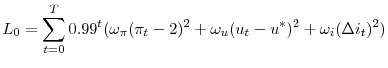
|
In this expression, πt denotes the inflation rate in quarter t (defined as the four-quarter percent change of the PCE deflator), ut the unemployment rate, u* its longer-run normal value, and Δit the first difference of the federal funds rate. Because all three arguments in this loss function are squared, losses equal zero only when inflation is at 2 percent, the unemployment rate is at u*, and the nominal federal funds rate is constant; otherwise, losses are positive. Because policymakers have only one instrument to hit three targets, losses are almost inevitable although they can be minimized by selecting the appropriate interest rate path.
This loss function embeds a number assumptions. The objectives of policy are to stabilize inflation around 2 percent and the unemployment rate around u*. For the baseline case, we assume equal weights on both arguments. This formulation may be seen as consistent with the Federal Reserve's mandate to promote maximum employment and price stability--where the latter has been judged consistent with 2 percent inflation by the FOMC--while the term penalizing changes in the federal funds rate reflects a desire to avoid abrupt changes in the policy instrument.9 The objective function is symmetric around the target values, in that a given deviation of one variable to one side of its target value is as costly as the same-sized miss to the other side. In addition, future losses are discounted at a quarterly rate of 1 percent; thus, a given loss projected to occur 40 quarters into the future (such as a one-percentage-point departure of the unemployment rate from its longer-run normal value) is only two-thirds as costly as the same-sized loss incurred in the current period.As all the baselines used in our analysis assume that the economy converges over time to a long-run equilibrium in which the inflation rate is 2 percent, the unemployment rate settles at u*, and the federal funds rate remains constant at its longer-run value, beyond a certain point (called T in the above summation) expected losses are zero. Thus, we evaluate the loss function for only 20 years into the future, sufficient time for the economy to have essentially settled back into its long-run equilibrium.10
The remaining ingredient needed to compute an OC interest rate path is an initial projection for the economy that summarizes, among other things, the exogenous forces expected to affect the economy over the optimization horizon. For illustrative purposes, we begin by constructing a model forecast that starts in the third quarter of 2012 and is consistent with the SEP projections of real activity, inflation, and the federal funds rate made by FOMC participants at the time of its September 2012 meeting.11 This time period is of interest in part because it corresponds with that used to generate the OC policy path reported in a speech given by then Vice-Chair Yellen in November of that year.12 For the unemployment rate, PCE price inflation, core PCE price inflation, and real GDP growth, the initial projection matches the midpoint of the central tendency reported in the September 2012 SEP for the years 2012 through 2015; thereafter, these variables converge to the midpoints of the central tendency of their longer-run values. Similarly, the initial projection for the federal funds rate matches the median projection from the September 2012 SEP at year-end 2012 to 2015 (adjusted to a quarterly average basis), and thereafter converges to the median projection of its longer-run normal value.13
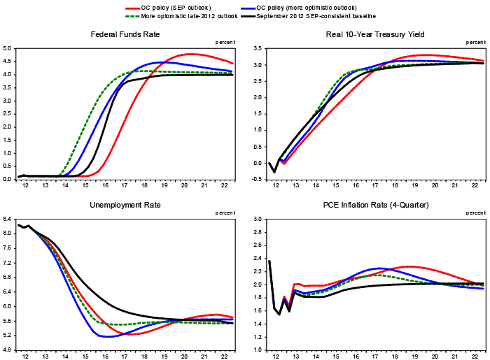
Figure 1 presents two sets of paths for the federal funds rate, the real yield on 10-year Treasury notes, the unemployment rate, and 4-quarter PCE inflation--one consistent with the September 2012 SEP and one based on OC policy. In both cases, the real 10-year Treasury yield at each point in time is calculated to be consistent with the relevant (perfectly-anticipated) paths of the federal funds rate and inflation over the next 10 years, plus an assumption about the evolution of the term premium beyond late 2012; because spending decisions in FRB/US depend importantly on longer-term real interest rates, the real 10-year Treasury yield is a useful indicator of the transmission of monetary policy to real activity and inflation. In the OC policy simulation we assume that the loss function weights on the three terms are all equal to 1.
| Figure 1: Predicted Outomes Under OC Policy Starting in Late 2012 |
|---|
 |
Starting from its initial level of 8 percent in the third quarter of 2012, the unemployment rate in the SEP baseline was projected to decline monotonically to its longer-run normal value over the coming six or so years. PCE inflation, measured on a 4-quarter basis, was expected to rise from about 1 1/2 percent in 2012 to about 1 3/4 percent in early 2013, and thereafter to gradually converge to 2 percent from below. The federal funds rate was projected to remain near zero until early 2015 and then to rise to close to its longer-run normal value of 4 percent by late 2016. By contrast, the OC path for the federal funds rate lifts off from the zero lower bound in early 2016. The real 10-year Treasury yield under this policy runs below the baseline path from late 2012 until late 2016, reflecting both the lower path of nominal short-term rates until 2018 and moderately higher inflation expectations over the 10-year window. These more-accommodative financial conditions are associated with an unemployment rate path that declines more rapidly than in the baseline, while inflation runs closer to the 2 percent goal on average.
Two results from this exercise are worth noting. First, along the optimal-control path, the federal funds rate lifts off from the zero lower bound three quarters later than in the baseline and continues to run below the baseline path for almost four years. Second, while the unemployment rate starts off well above its longer-run normal value and inflation below the FOMC's 2 percent objective, under OC policy both move to the opposite side of their respective long-run values for a while, whereas under the baseline outlook they converge monotonically to their longer-run values. This latter outcome reflects the commitment of policymakers to follow through with the policy path chosen in late 2012, and the assumption that this commitment is fully credible. Were policymakers to recalibrate policy in 2016 without any weight placed on the previously chosen policy path, they would not wish to follow through with the original plan as it entails inflation running above target for a time, accompanied by unemployment below its natural rate. From the perspective of late 2012, however, a promise to achieve this combination for a time in the future is desirable because it generates the financial conditions needed to make more-rapid progress over the near-to-medium term in reducing labor market slack. In other words, under the conditions expected as of late 2012, the predominant component of policymakers' loss under baseline conditions (assuming equal weights) is the elevated level of unemployment projected from late 2012 through 2015, and a large reduction in loss achieved by bringing about a more rapid recovery under OC policy outweighs the relatively small increase in loss incurred by the moderate undershooting of the unemployment rate and overshooting of inflation later in the decade.
Variations on the Baseline Case
We will now examine
how robust these results are to changes in certain aspects of the loss function,
the model, and the initial economic outlook. Starting with the loss function,
while its first two arguments--the concern for stabilizing inflation and the
unemployment rate around their respective target values--are suggested by the
Federal Reserve's dual mandate, it is not obvious that the weights
ωπ and ωu on these two elements should
be equal. In fact, loss functions of this form derived from explicit
welfare-theoretic considerations frequently suggest weights that are far from
equal, depending on a range of economic assumptions.14 Moreover,
concerns about the possible consequences of abrupt changes in short-term
interest rates do not help pin down the weight ωi with any
precision.
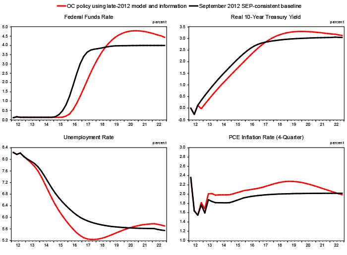
Figure 2 compares the OC interest rate path shown in Figure 1 to ones derived under three alternative choices of loss function weights. In the first alternative, we raise the penalty on unemployment rate deviations ωu to 10 while keeping the weights on inflation deviations and interest rate changes at 1; in the second, we raise the penalty on inflation deviations ωπ to 10 while keeping the other two weights at 1; and in the third, we reduce the weight on interest rate changes to 0.1, while assigning weights of 1 to inflation and unemployment rate deviations. The latter case may be viewed as a more direct representation of the dual mandate. Raising the weight on squared unemployment gaps calls for a federal funds rate path that postpones liftoff by three quarters relative to the OC path with equal weights, which is not surprising given the previously discussed dominance of the squared unemployment gap term in determining the overall losses incurred during the early years of the simulation. This policy achieves a somewhat more rapid reduction in the unemployment rate, together with a persistently higher path for inflation and a lower path for the real 10-year Treasury yield. Conversely, raising the weight on squared inflation gaps implies a relatively lower weight on unemployment rate gaps, and therefore leads to a somewhat higher funds rate path than under the baseline OC policy. In the simulation in which the weight on squared interest rate changes is reduced to 0.1, the federal funds rate lifts off from its lower bound three quarters later than under the baseline OC strategy, but then rises rapidly and overshoots the baseline path. As a result, the path in this case induces outcomes for the unemployment rate and inflation that are similar to the baseline case, indicating that, at least in this instance, the weight on interest rate changes doesn't constrain the pursuit of the dual mandate objectives in a meaningful way.15
| Figure 2: Sensitivity of Outcomes Under Late-2012 OC Policy to Changes in the Loss Function Weights |
|---|
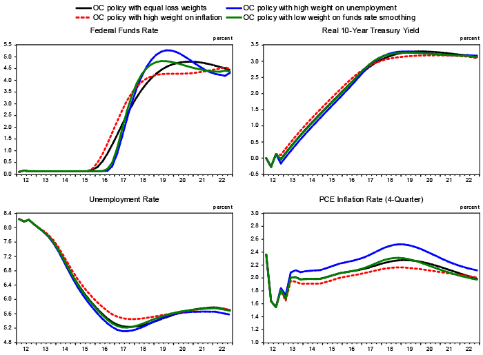 |
Figure 3 explores how alternative characterizations of the dynamics of the economy--specifically, alternative versions of the FRB/US model--can affect OC policy prescriptions. Since 2012, the FRB/US model has undergone several changes. The most notable of these is a re-specification of the model's wage-price block, which has decreased both the persistence and magnitude of the response of inflation to movements in economic slack. Because in FRB/US the response of inflation to movements in the funds rate operates through the effects of real interest rates on (current and expected future) slack, this change in the characteristics of the wage-price block reduces the response of inflation to movements in the funds rate. Thus, compared to the corresponding paths generated using the version of the model in place in late 2012, the OC path for the federal funds rate derived using the late-2014 version of the model rises less rapidly, resulting in a lower trajectory for unemployment as well as lower inflation late this decade.16
| Figure 3: Sensitivity of Outcomes Under Late-2012 OC Policy to Changes in the FRB/US Model |
|---|
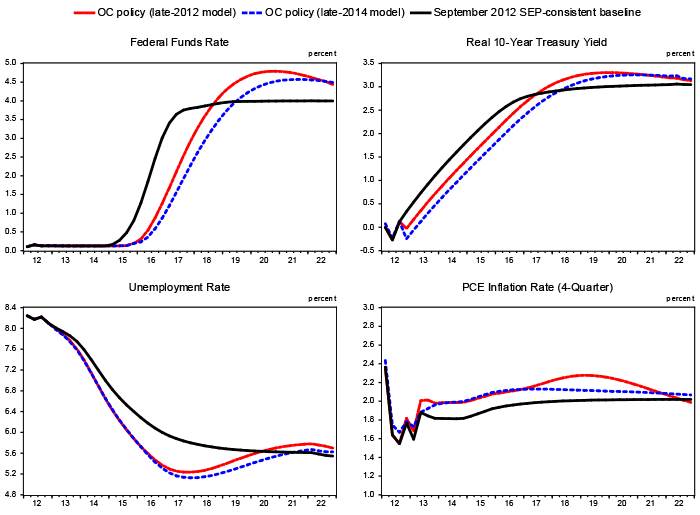 |
Figure 4 illustrates the relevance of the economic outlook for calculations of the optimal-control path. It compares paths for the variables under the baseline outlook as of September 2012 (the black lines) with a set of paths for a more optimistic baseline that features a more rapid decline in the unemployment rate similar to that observed over the past two years (the green lines). The red lines and blue lines show the OC paths corresponding to these two alternative outlooks, both computed using the 2012 version of the model. As can be seen, the OC policy that anticipates the surprisingly rapid decline of the unemployment rate in 2013 and 2014 lifts the funds rate off the zero bound earlier and then keeps it higher for several years relative to the OC policy based on the outlook in the 2012 SEP. From 2015 to 2018, the unemployment rate runs below the longer-run normal rate while inflation rises modestly above 2 percent, outcomes that only obtain if the public expects policymakers not to reoptimize at that time. The figure thus illustrates two different potential reasons for changes to previously announced policy plans: Policymakers could choose a new policy path in response to unanticipated changes in the economic outlook, as is the case in figure 4; or they could do so because they do not wish to follow through on previously made commitments. Only in the latter case would the benefits of commitment policies disappear.
| Figure 4: Sensitivity of OC Policy to Changes in the Economic Outlook (results computed using the late-2012 version of the FRB/US model) |
|---|
 |
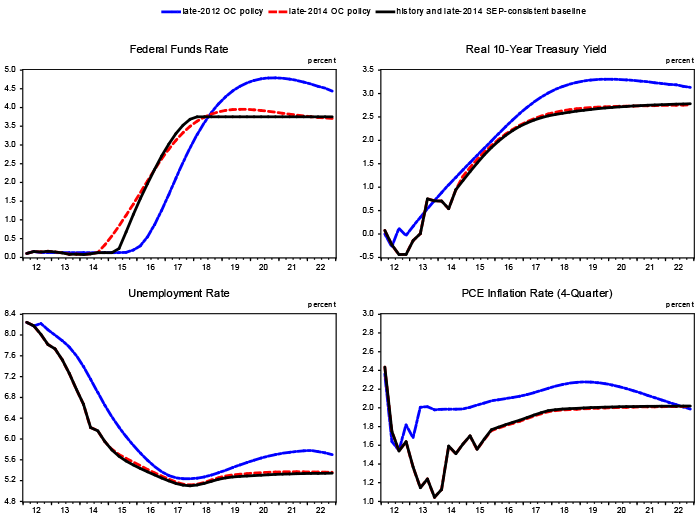
Finally, Figure 5 shows the OC paths as of late 2014, using the 2014 model and September 2014 SEP outlook, and compares them to the optimal paths shown in Figure 1, based on the September 2012 outlook and the version of the model then in use. This comparison provides an impression of how OC paths can change over time in response to the arrival of new information (about exogenous forces affecting the economy or about its structure) as well as the fact that this reoptimization does not take account of previous commitments. In the OC paths as of late 2014, the federal funds rate lifts off from the zero lower bound before the contemporaneous SEP-consistent baseline does, in contrast to the results from late 2012.17 While the unemployment rate declines below its longer-run normal value of 5.35 percent for a couple of years, this undershooting is now quite modest, and, given the inertial behavior of inflation, is associated with an inflation path that converges monotonically from below to the 2 percent objective. Thus, the inflation overshooting and other features of the optimal-control paths highlighted in figure 1 are not intrinsic to OC policy at the zero lower bound, but are instead dependent on the trade-offs inherent in the model and the initial conditions.
| Figure 5: OC Policy and Predicted Outcomes -- Late-2012 Estimates Versus Late-2014 Estimates (estimates derived using the information and model version available at the time of the OC calculation) |
|---|
 |
Conclusions
Given the objectives for monetary policy, a characterization of the dynamics of the economy as embedded in a model, and a view about the exogenous forces shaping the outlook, optimal-control paths for the federal funds rate can be generated to help inform monetary policy decisions, supplementing other benchmarks such as prescriptions from simple interest rate rules. Compared to the latter, OC policies afford greater flexibility in making commitments to future policy responses conditional on economic conditions. Such commitments are particularly valuable when the policy instrument is constrained by the zero lower bound. However, as illustrated in this Note, OC paths are sensitive to the specific assumptions used in their computation. Thus, different assumptions about the economic outlook or the dynamics of the economy can lead to different results; for example, the FRB/US-based estimates reported here would look different if we had instead employed a model with a different characterization of, say, the way in which firms and households form their expectations of future economic developments, or the role of financial intermediation and financial frictions in the economy. Moreover, the OC paths illustrated in this Note are based on the notion that policymakers will not re-run the optimization process at a later date, whereas in reality policymakers reconsider earlier decisions continually in light of new information. Thus, OC paths should be treated with appropriate caution as a guide to actual policy.
References
Brayton, Flint, Eileen Mauskopf, David Reifschneider, Peter Tinsley, and John Williams, 1997. "The Role of Expectations in the FRB/US Macroeconomic Model." Federal Reserve Bulletin, April, 227-245.
Chung, Hess T., Edward Herbst, and Michael T. Kiley, 2014. "Effective Monetary Policy Strategies in New-Keynesian Models: A Re-Examination." NBER Macroeconomics Annual, forthcoming.
English, William B., David Lopez-Salido, and Robert Tetlow, 2013. "The Federal Reserve's Framework for Monetary Policy – Recent Changes and New Questions," Federal Reserve Board, Finance and Economics Discussion Series 2013-76.
Henderson, Dale, and Warwick J. McKibbin, 1993. "A comparison of some basic monetary policy regimes for open economies: implications of different degrees of instrument adjustment and wage persistence (PDF)," Carnegie-Rochester Conference Series on Public Policy, vol. 39 (December), pp. 221-317.
Orphanides, Athanasios, and John C. Williams, 2008. "Learning, Expectations Formation, and the Pitfalls of Optimal Control Monetary Policy (PDF)," Journal of Monetary Economics, vol. 55 supplement (October), pp. 580-96.
Svensson, Lars E.O., and Robert J. Tetlow, 2005. "Optimal Policy Projections (PDF)," International Journal of Central Banking, vol. 1 (December), available at http://www.ijcb.org/journal/ijcb05q4a6.htm.
Svensson, Lars E.O., and Noah Williams, 2007. "Bayesian and Adaptive Optimal Policy Under Model Uncertainty (PDF)," National Bureau of Economic Research Working Paper No. 13414 (September).
Taylor, John B., 1993. "Discretion versus Policy Rules in Practice (PDF)," Carnegie-Rochester Conference Series on Public Policy, vol. 39 (December), pp. 195-214.
Taylor, John B., and John C. Williams, 2011. "Simple and Robust Rules for Monetary Policy (PDF)," in Benjamin M. Friedman and Michael Woodford, eds., Handbook of Monetary Economics, vol. 3B, (San Diego: North Holland), pp. 829-60.
Woodford, Michael, 2003. Interest and Prices: Foundations of a Theory of Monetary Policy. Princeton, NJ: Princeton University Press.
Yellen, Janet L., 2012. "Revolution and Evolution in Central Bank Communications," speech delivered at the Haas School of Business, University of California at Berkeley, November 13.
1. For example, see Charts 8 and 9 in the "Bluebook (PDF)" prepared for the December 15-16, 2008 FOMC meeting. Return to text
2. Simple interest rate rules were first popularized by Henderson and McKibbin (1993) and Taylor (1993). For a recent overview and evaluation of simple interest rate rules, see Taylor and Williams (2011). Return to text
3. Some simple rules, however, are in principle able to deliver expectational effects similar to those achieved by OC policy under conditions of protracted economic weakness and near-zero policy rates. For example, model simulations presented in English et al. (2013) and Chung et al. (2014) suggest that if a central bank were to respond to such a situation by credibly committing to following a nominal income targeting rule in the future, then expected future inflation would rise, leading to a reduction in real interest rates today and so stimulating aggregate demand. Return to text
4. For a further discussion of these and other limitations of OC policies, see Orphanides and Williams (2008), for example. Return to text
5. For a more technical exposition of the concept of optimal-control policy paths constructed around an initial projection derived using judgmental or other non-model information, see Svensson and Tetlow (2005). Also, see Svensson and Williams (2007) for an example of how to use more than one model in an OC exercise to hedge against possible specification errors in characterizing the dynamics of the economy. Return to text
6. Documentation of the model is available at www.federalreserve.gov/econresdata/frbus/us-models-about.htm, including a complete listing of model equations and coefficients, papers discussing different aspects of FRB/US, as well as the complete model code and illustrative simulation programs, including sample code for optimal control policy. The specific programs and databases used to generate the results reported in this Note are available upon request from the authors. Return to text
7. Specifically, we assume that financial market participants and wage-and-price setters have a complete understanding of both policy and the dynamics of the FRB/US model, implying that their expectations are rational in the sense of being fully model-consistent (MCE). In contrast, the expectations underlying the spending and capital investment decisions of households and non-financial firms are assumed to be based on the limited information and average historical relationships embedded in the predictions of a small-scale VAR model, on the grounds that these agents (especially households) are typically less informed about both policy and the workings of the economy. The transmission of monetary policy depends on these assumptions, and hence alternative choices in this regard would lead to different results. For a detailed discussion of the assumptions with which expectations are modeled in FRB/US, see Brayton et al. (1997). Return to text
8. See, for example, Woodford (2003) chapter 7 for a discussion of the benefits of commitment. Under certain economic conditions, commitment policies that are viewed as credible can yield policy paths that are quite different from, and associated economic outcomes that are significantly better than, those associated with discretionary strategies that optimize period by period. Return to text
9. The interest-rate-smoothing term primarily serves to prevent unrealistic outsized quarter-to-quarter movements in short-term interest rates in the simulation, rather than reflecting an actual preference on the part of policymakers. As will be demonstrated below, this basic objective is achieved in OC simulations even if the relative importance placed on interest rate smoothing is quite low. Return to text
10. Although not shown in formula, the loss functions used in our analysis also include another term that sharply penalizes movements in the nominal funds rate below 12 1/2 basis points; adding this term allows us to impose an effective floor on nominal interest rates consistent with the zero lower bound. Return to text
11. The SEP is an addendum to the FOMC minutes. The September 2012 SEP is available at Board of Governors of the Federal Reserve System (2012), "Minutes of the Federal Open Market Committee, September 12-13, 2012, (PDF)" press release, October 4. Return to text
12. See Yellen (2012). The baseline projections used in that speech were constructed to match the primary dealers' projections as reported in a survey conducted by the Federal Reserve Bank of New York, not the September 2012 SEP forecasts. Return to text
13. The longer-run values for the unemployment rate and the real short-term interest rate implied by the September 2012 projections are u* = 5.6 percent and r* = 2.0 percent. Return to text
14. See, for example, Woodford (2003) chapter 6 for a derivation of loss functions based on a second-order approximation of households' welfare. While the derived loss functions are of the quadratic form considered here, various arguments can be made for loss functions that are not symmetric around the inflation target π* and the natural rate u*. For example, unemployment below its natural rate may have lower welfare costs relative those incurred when u>u*.Return to text
15. Although not shown, modest variations in the discount rate used to compute overall losses--including computing losses without any discounting--also have little effect on outcomes under OC policy. Return to text
16. Of course, larger differences than those shown in figure 3 can result if OC paths are computed using models whose specifications of inflation dynamics and other features of the economy differ more substantially from the 2012 version of the FRB/US model. For a discussion of the appreciable sensitivity of predicted monetary policy effects to different specifications of price setting, see Chung et al. (2014). Return to text
17. This result, however, is driven by the penalty on interest rate changes in the loss function. For a weight of 0.1 on interest rate changes, liftoff occurs in the same quarter as in the baseline. Return to text
Please cite as:
Brayton, Flint, Thomas Laubach, and David Reifschneider (2014). "Optimal-Control Monetary Policy in the FRB/US Model," FEDS Notes. Washington: Board of Governors of the Federal Reserve System, November 21, 2014. https://doi.org/10.17016/2380-7172.0035
Disclaimer: FEDS Notes are articles in which Board economists offer their own views and present analysis on a range of topics in economics and finance. These articles are shorter and less technically oriented than FEDS Working Papers.
