Skip to: [Printable Version (PDF)] [Bibliography] [Footnotes]

Finance and Economics Discussion Series: 2008-43 Screen Reader version ^♣

Distress in the Financial Sector and Economic Activity

Mark Carlson, Thomas King, Kurt Lewis*

Board of Governors of the Federal Reserve, Washington, DC 20551

Keywords: Bank distress, economic activity, financial intermediation

Abstract:

This paper explores the relationship between the health of the financial sector and the rest of the economy. We develop an index of financial sector health using a distance-to-default measure based on a Merton-style option pricing model. Our index spans over three decades and appears to capture periods when financial sector institutions were strong and when they were weak. We then use vector autoregressions to assess whether our index of financial-sector health affects the real economy, in particular non-residential investment. The results indicate that our index has a considerable impact. Moreover, we find that this financial channel amplifies changes in investment resulting from shocks to non-financial firm profitability.

JEL: E44, E50, G20

Preliminary
Please do not cite without permission

1 Introduction

The financial sector of the economy, by facilitating the flow of funds from investors to borrowers, is an important contributor to economic growth. Disruptions that interfere with the ability of the financial sector to intermediate financial flows might therefore be expected to restrain economic activity. In particular, it is possible that a deterioration in the health and the solvency of financial institutions might raise the cost of intermediation. In the extreme case, the failure of a financial institution, valuable banking relationships are lost and firms may find their access to credit restricted and their ability to invest reduced. Bernanke (1983) argues that this mechanism played a role in the economic collapse of the Great Depression. Even in the less extreme cases in which bank health deteriorates but does not end in failure, one might expect intermediation costs to increase. For example, in the model developed by Goodhart, Sunirand, and Tsomocos (2006), deposit and loan rates increase and borrowing activity declines as banks move close to violating their capital adequacy requirements.

This idea is distinct from, but complementary to, the literature investigating the role of the "financial accelerator" in macroeconomic performance (e.g., Bernanke, Gertler, and Gilchrist (1999); Bernanke and Gertler (1989)). In these models, savers are the source of funds, firms need to borrow these funds, and intermediaries help transfer the funds from savers to firms. In these models, there is a friction, such as asymmetric information, that increases the cost to a firm of external finance from an intermediary relative to internal finance. A financial institution provides a contract that solves this asymmetric information problem, but firms pay an endogenous premium for external finance. Dynamics in these models are driven by shocks to the condition of the borrower. Financial intermediaries in these models are passive but play a crucial role. Our work builds on the idea that these financial institutions could also be the source of important dynamics. The financial intermediaries are themselves dependent on debt financing, so that if their condition deteriorates they will face higher borrowing costs which may be passed on to borrowing firms. Higher lending rates would increase external finance premia and affect investment decisions even for borrowers of unchanged quality. In other words, financial-sector health itself should partially determine whether the financial accelerator is economically important.

This paper investigates the impact of changes in the health of financial intermediaries on capital investment on a macroeconomic level. To do so, we use a Merton asset pricing framework to develop a measure of the distance to default for large financial institutions in the United States, including both commercial and investment banks, from 1973 through 2007. Although one might question the ability of the Merton framework to accurately measure construct default probabilities of highly leveraged institutions, the relative movements in our measure appear reasonable both in the aggregate and for individual institutions. Thus, we take this measure as a reasonable index of market concern about the health of financial institutions.

We then test whether this index is related to the macroeconomy. We start by testing whether changes in our measure of financial sector health are related to changes in lending standards and terms. We find that changes in our measure Granger cause change in lending standards and terms as reported in the Federal Reserve Senior Loan Officer Survey of Bank Lending Practices. This finding suggests that bank health may be a factor in determining the ability of nonfinancial firms to obtain credit.

Using vector autoregressions (VARs), we then test whether our measure affects aggregate capital investment by nonfinancial firms. We focus especially on the impact on investment spending, as the channel by which the borrowing costs of nonfinancial firms might be affected is fairly clear. When conducting the VARs we include several control variables, such as corporate profits and corporate bond spreads, that might also affect investment spending. This analysis builds on the recent work by Aspachs, Goodhart, Tsomocos, and Zicchino (2007). Their work points to a link between the health of the financial sector and GDP growth, but their analysis has been limited to a fairly recent period. Having more than three decades of data provides us with a relatively rich time series to analyze the interaction of financial sector health and other parts of the economy.

We find that the health of the financial sector does indeed have an impact on macroeconomic variables. A typical negative shock to our index results in a cumulative decrease in investment of about 2 percent over the subsequent two years. Further, we find that the impact of shocks to the profitability of nonfinancial firms on investment is magnified by the inclusion of financial variables in the VAR. This effect occurs because declines in firm profitability decrease the health of the financial sector which in turn have their own impact on investment, an amplification mechanism reminiscent of the mechanisms in the financial-accelerator literature.

The paper proceeds as follows. In Section 2, we motivate our empirical research by reviewing some of the theoretical and empirical research investigating the linkages between bank health, the costs faced by firms, and their investment decisions. Section 3 discusses the creation of our measure of the health of financial institutions. The measure provides a picture of the relative health of the U.S. financial sector over time is interesting in its own right. The results of our tests relating our distance to default measure to the real economy are discussed in Section 4. Section 5 concludes.

2 Motivation

Our empirical research is motivated by the idea that a change in the health of a financial intermediary (hereafter, "bank") will affect its borrowing costs and lending rates and/or lending standards. A decline in the health of the bank will increase its borrowing costs. A deterioration in bank health may also lead the bank to charge higher rates on the loans it makes, especially if the bank needs to pay more on deposits. The bank may also respond to a deterioration in its condition by tightening lending standards as lower loan losses might allow it to rebuild its capital.¹ As credit conditions tighten and the cost of credit increases, nonfinancial firms scale back their investment and economic activity may be restrained.

This argument has been developed in a number of recent theoretical papers. Goodhart, Sunirand, and Tsomocos (2005) and Aspachs, Goodhart, Tsomocos, and Zicchino (2007) provide an intricate model of the banking sector involving differentiated banks, an interbank market, a loan market, and choice of repayment by individual banks. In these models, they discuss the impact of an increase in capital adequacy requirements on the banking system. The bank responds by increasing its risk profile which, in equilibrium, raises the rates that it must pay depositors and, as a profit maximizer, the rates that it charges on loans. (Banks may be able to pass these costs on to borrowers in part because of difficulty on the part of borrowers in switching banks. See, for instance Rajan (1992) for a discussion of the costs of switching lenders.) Higher borrowing costs leads to reduced borrowing and lower economic activity. A model providing the connection between bank condition and lending standards is presented by Gorton and He (2005). They argue that information about loan losses provide other banks information about the lending standards of other banks and that larger loan losses lead to tighter lending standards. These tighter lending conditions in turn reduce borrowing and reduce economic activity.²

There are other theoretical papers that articulate feedback loops between the financial sector and a production economy. Bauducco, Bulir, and Cihak (2008) develop a model in which changes in interest rates can influence the probability that borrowers from a bank default and thus the amount of credit the bank extends. von Peter (2004) develops an overlapping generations model in which falling asset prices increase firm defaults which, in turn reduce the ability of banks to extend credit. The reduction in bank credit can spill back into asset prices.

There is also considerable previous empirical support for the notion that the health of the financial sector matters for real economic activity and investment in particular. Some of this evidence is from studies of individual institutions. Evidence that banks in poorer financial health charge more for loans comes from Hubbard, Kuttner, and Palia (2002), who, using data on syndicated loans, find that less well capitalized banks tend to charge higher loan rates than well capitalized banks. Bank health has also been found to affect investment. Studies of Japanese banks in the 1990s, such as Gibson (1995), have shown that declines in the health of the banks resulted in lower investment on the part of their Japanese customers. Further, Peek and Rosengren (2000) find that the deterioration in the position of Japanese banks reduced activity in the U.S. commercial real estate markets that were dependent on Japanese bank lending. In work exploring the response of investment to changes in financing costs, Guiso, Kashyap, Panetta, and Terlizzese (2002) find that measures of bank health--as well as bank size, efficiency, and market share--are useful instruments for the interest rate that banks charge on their loans. They further find that investment responds fairly strongly to changes in financing costs.

There has also been some work at a more aggregate level suggesting that a serious deterioration in bank health has a macroeconomic impact. Bernanke (1983) looks at the experience of the United States in the Great Depression and finds that bank failures decreased economic activity. More recently, Aspachs, Goodhart, Tsomocos, and Zicchino (2007) use a vector autoregression involving GDP growth, inflation, bank profitability, and a measure of the probability of bank default. They find that increases in the probability that banks default have a negative effect on GDP growth.

One channel by which we believe a deterioration in bank health affects borrowing conditions is by causing banks to tighten lending standards. Lown, Morgan, and Rohatgi (2000) analyze the impact of the share of loan officers reporting in the Federal Reserve's Senior Loan Officer Opinion Survey of Bank Lending Practices that they had tightened their lending standards on output. They find that tighter lending standards reduced loan growth and has predictive power for output growth. Thus, if a deterioration in the condition of banks causes banks to tighten their lending standards, this channel might be another through which bank health affects investment.

Thus, there is a variety of evidence at both the microeconomic and macroeconomic level that suggests that the health of the financial sector ought to matter for economic activity. While this evidence is wide ranging, it has tended to focus on particular episodes in which the condition of the banking sector deteriorated notably. Even the study by Aspachs, Goodhart, Tsomocos, and Zicchino (2007) uses a measure of the probability of default that is zero unless it crosses a relatively high threshold. (Lown, Morgan, and Rohatgi (2000) look over a longer period, but do not focus on the overall health of financial institutions.) This paper builds on this previous research by looking at a much longer time frame for systematic effects of changes in the health of the financial system on the real economy, in normal times as well as in crisis periods. To do so, however, we first need a measure of financial-sector health.

3 An index of financial sector health

We construct a measure of the distance to default for a sample of financial institutions based on a Merton asset pricing model Merton (1974). This method uses the difference between market value of a firm's assets and its liabilities and the volatility of the value of assets to provide a measure of how close a firm is to having liabilities exceed assets. The sample of institutions used in our analysis includes large commercial banks, investment banks, and other financial intuitions. Thus, our measure is more likely to reflect the condition of the broad financial system than if the measure included only commercial banks. We are able to calculate our measure of the distance to default back to 1973, providing us with a relatively long time series.

3.1 Data and methodology

Using data from Compustat, we select the 25 largest financial institutions by assets in each quarter since 1973. These financial institutions are limited to depository institutions, non-depository credit institutions, securities and commodity brokers and dealers, and their holding companies.³ There are roughly 70 separate firms that are included in the top 25 firms in at least one quarter (these firms are listed in Appendix A). We match the quarterly balance sheet data from Compustat for all the institutions in our list to daily data from CRSP on stock prices and equity shares outstanding.

To calculate a our measure of distance to default, we need information on liabilities, the market value of assets, and the volatility of the market value of assets. We are able to obtain information on total liabilities from Compustat (in particular we use total liabilities and linearly interpolate between quarterly reporting dates). To compute the market value of assets and the volatility of the market value of assets, we use the formulas based on Black and Scholes (1973) and Merton (1974) as described in Crosbie and Bohn (2003). In particular, the market value of a firm's equity at time , , can be thought of as a call option on the market value of a firm's assets, , with a strike price equal to the current book value of the firm's debt, . Using the Black and Scholes formula:

$\displaystyle {E_t} = {V_t} N(d_1)- e^{r_t T}{D_t} N(d_1 - \sigma_{V_t} \sqrt{T})$

(1)

where

is the risk free interest rate,

is a measure of the time horizon of interest, $\sigma_V$ , is the volatility of the market value of assets,

represents the cumulative normal distribution, and

is the delta of the option:

$\displaystyle {N(d_1)} = N(\frac{ln(\frac{V_t}{D_t}) + (r+\frac{\sigma_{V_t}}{2})T}{\sigma_{V_t} \sqrt{T}})$

(2)

The market value of the firm's equity is also observable, but the market value of assets and the volatility of that market value are not. However, asset volatility can be estimated using the relationship between asset and equity volatility, $\sigma_E$ , from the Black-Scholes model:

$\displaystyle {\sigma_{E_t}} = \frac{V_t}{E_t} N(d_1) \sigma_{V_t}$

(3)

Equations 1 and 3 can be solved jointly for

and $\sigma_V$ . Following much of the literature, we focus on a one-year time horizon. For the risk free rate, we use the one-year Treasury rate.

Often $\sigma_E$ is computed from equity options. However, these options are not available for much of our sample period. As a substitute, for each firm , we use exponentially weighted realized volatilities:

$\displaystyle {\sigma_{E_{it}}} = \frac{\sum_{s=1}^{t}{ e^{-\alpha_i (t-s)}(x_{is} - \mu_{is})^2}}{\sum_{s=1}^{t}{ e^{-\alpha_i (t-s)}}}$

(4)

where $x_{it}$ is firm

's return in day

, $\mu_i$ is its average return over the sample, and $\alpha_i$ is a firm-specific smoothing parameter to be estimated. To determine the optimal choice of $\alpha_i$ for each institution, we follow the procedure of Foster and Nelson (1996).⁴ These authors derive a formula that maps the variance of the daily changes in volatility into an optimal choice for $\alpha_i$ . In practice, this variance can be estimated by guessing a value for $\alpha_i$ and computing the volatility sequence $\sigma_{i1}^2,\cdots,\sigma_{i\tilde{T}}$ using the above equation. The Foster-Nelson formula then provides a new value $\alpha_i$ , and the procedure can be iterated until convergence.

Similar to Liu, Papakirykos, and Yuan (2006), we use a Z-score as our measure of the distance to default: We calculate this measure as:

Distance to default $\displaystyle = \frac{\frac{V_t-D_t}{V_t}}{\sigma_{V_T}}$

(5)

Using the entire stock price history of each firm from 1973 (or initial public offering date) to year-end 2007 (or the date the firm's equity stopped trading), we calculate the expected probability of default on a daily basis. We then extract the 25 largest firms, by assets, in each quarter and calculate their expected default probability. The median default probability of the top 25 firms serves as our expected default measure. We use the median because it is more likely reflects the general condition of the financial institutions in our sample. A sizable increase in the median is likely to reflect a change in the distance to default measure for many of our firms. Nevertheless, we have tried alternative weighting schemes and resulting measure is not materially different from the median in most cases.⁵ We convert the daily measure to a monthly or quarterly frequency by averaging it over the relevant time period.

The institutions that constitute the largest 25 institutions shift over time. These changes occur as institutions merge and as the relative size of institutions changes. These shifts tend to occur gradually; the average number of new firms each quarter is 0.77 (i.e. there are about three changes to the panel in a year). Thus, we argue that our measure is broadly comparable over time.

Commercial banks account for roughly two-thirds of the institutions included in the sample. Over time, the share of institutions in the top 25 that consist of non-commercial banks edged higher from four in the first years of the sample to eight at the end of the sample. To investigate the implications of these compositional shifts, we calculated the distance to default measure separately for commercial banks and non-commercial banks (using the median of the twelve larges institutions in each group). The resulting two time series have a correlation coefficient of .84. The median distance to default is a bit closer to zero (default) for non-commercial banks, but the difference is not large. Moreover the difference diminishes during the latter half of the sample period when non-commercial banks constitute a larger part of the sample of institutions used to construct our measure.

Other researchers have used similar measures based on default probability.⁶ These indexes are generally constructed in a somewhat similar fashion to the one constructed here, although they tend to focus almost exclusively on commercial banks and cover notably shorter periods. Gropp, Vesala, and Vulpes (2006) construct a distance to default measures for large European banks from 1991 to 2001 based on equity values and compare it to subordinated debt spreads. They similarly use a measure of realized volatility, in particular a six-month moving window. They find that their measure predicts rating downgrades to below "C" in the Fitch/ABCA individual rating (which excludes the impact of a government safety net). Chan-Lau and Sy (2007) propose a distance to capital, based on the idea that banks are closed before equity has completely disappeared. Basurto, Goodhart, and Hofmann (2006) use a probability of default measure for banks in a sample of OECD countries and explore whether a range of financial and real factors explain such probabilities of default over time.

3.2 Behavior of the index

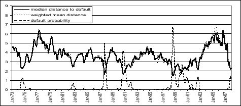
Our measure of the median distance to default is shown in Figure 1 by the black line. For comparison with alternative weightings of institutions we also include the mean distance to default weighted by assets (the green line). We also convert the median distance to default to a probability of default using a cumulative normal distribution (Probability of default = $\Phi$ (-Distance to default)). This nonlinear transformation makes periods of stress stand out which makes looking at the behavior of the measure a bit easier. However, in our analysis relating the health of the financial sector to the real economy we prefer the distance to default measure which exhibits less extreme movements.

The behavior of our measures appears quite reasonable. During periods when there was concern about the health of the financial sector, the distance to default measure moves closer to zero and the probability of default measure increases. The earliest period of distress appears in 1974, around the time of the Herstatt and Franklin National bank failures.⁷ There is also increase in the probability of default measures around the time of the 1987 stock market crash.⁸ The distance to default measure approaches zero in the early 1990s around the time when bank profitability was low, there was an elevated number of bank defaults, and there were concerns about a credit crunch. Our measure of the distance to default also stays closer to zero for longer in this episode than most proceeding ones. The troubles in the financial sector following the Russian default and troubles at Long Term Capital Management in 1998 represent the largest rise in the expected probability of default. Concerns about the financial sector, at least according to our measure, persisted for a while as the financial sector was affected by the declines in equity markets in 2000 and the WorldCom default in 2002.

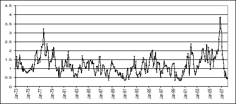
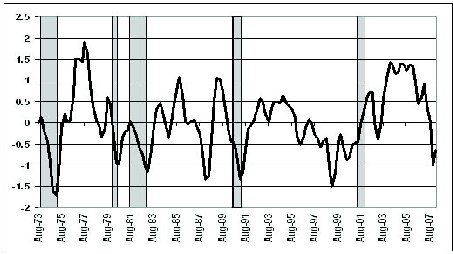
**Figure 1:** Measure of default risk in the financial sector
(monthly) Figure 1 Data

In addition to looking at the median expected default probability, we can also look at the difference between the 75th and 25th percentiles of the distribution of firm distances to default. The time series of this difference is shown in Figure 2. Interestingly, we find that largest difference in the quartiles during periods when there was the least concern about the health of the financial sector (when the distance to default was furthest from zero). Conversely, during periods of heightened concern about the financial sector, the interquartile range is generally relatively small. These results suggest that, when our measure indicates an elevated level of concern about the financial system, it tends to reflect concerns about the broad financial sector, rather than about individual institutions.

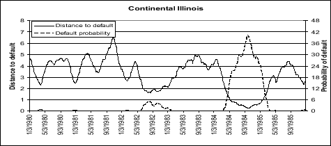
**Figure 2:** Interquartile range of the distance to default measure
(monthly) Figure 2 Data

Gropp, Vesala, and Vulpes (2006) find that distance to default measures do appear to predict troubles at financial institutions; it is interesting to look at a particular instance to see how quickly the measure moves and how large these movements are. We look at changes in our measure for Continental Illinois between 1979 and 1985 (shown in Figure 3). In addition to the distance to default, we also show the implied probability of default. The measure appears to capture market concerns quite well. There is a decline in the measures of the distance to default and an uptick in the probability of default in 1982, around the time of the failure of Penn Square, a bank that had sold Continental Illinois a number of bad loans. Default expectations also increase sharply in 1984 around the time of the bank run on May 8, 1984. Default concerns continued to rise over the next few months and only decreased around the time of the approval of the FDIC rescue plan by the shareholders of Continental Illinois Corporation on September 26, 1984.⁹

**Figure 3:** Measure of default risk for Continental Illinois
(daily) Figure 3 Data

The distance to default measure resulting from our calculations should not be taken literally. One reason is that these institutions, especially the commercial banks, are likely to be closed by financial regulators prior to the complete erosion of capital. Thus, the default condition is not the one assumed in the Merton model (see Chan-Lau and Sy (2007) for further discussion of this issue). The model also assumes risk neutrality, which is also unlikely to hold.¹⁰ Nevertheless, since the timing of movements in the distance-to-default measure at both the individual and aggregate level appear to correspond to events that would be expected to affect concerns about the financial sector, we take our measure as a reasonable proxy for market concerns about financial sector health.

4 Financial-sector health and the real economy

In this section, we present the results of our investigations into whether our measure of financial sector affects the real economy. As discussed above, our motivation is that distress at financial institutions may cause these institutions to restrict the flow of credit and thus may hinder economic performance. As an preliminary step, therefore, we test whether changes in our index do indeed lead to changes in bank lending standards and terms. We then use vector autoregressions to test whether the index is related to investment.

4.1 Impact on lending standards and terms

We expect that the health of financial institutions to matter because it will lead banks to tighten lending terms and/or standards. We test this hypothesis using data from the Federal Reserve Senior Loan Officer Opinion Survey of Bank Lending Practices from 1990 through 2007. In this survey, banks are asked about whether they have changed their lending standards or terms to their large business borrowers customers.¹¹ In each quarter, the Federal Reserve reports the net share of banks that reported tightening standards and the net share reporting tightening terms during the preceding three months (net shares are the share that reported tightening minus the share that reported easing).

We look at whether changes in our measure of financial sector health Granger causes changes in lending standards or terms. As shown in Table 1, we find that it does indeed Granger cause changes in lending standards. Our measure and changes in lending terms appear to Granger Cause each other (Table 2). These results are broadly consistent with the reports of banks themselves. Banks are asked on the Senior Loan Officer Opinion Survey about the reasons that they changed their lending standards or terms. At times, banks have reported that a deterioration in their capital position was a reason for tightening credit conditions. The findings also are consistent with our hypothesized channel by which a deterioration in bank health can restrain nonfinancial investment.

4.2 Direct impact of financial sector health on the real economy

To investigate the importance of the financial sector in initiating and propagating shocks to the real economy, we estimate vector autoregressions (VARs) over real and financial variables, including our index of financial-sector health.¹² We focus on corporate capital investment, which we take to be determined largely by firm profitability and borrowing costs.

The variables included in our VAR are non-financial after-tax profits from the NIPA data, deflated by the GDP deflator; real nonresidential fixed investment; the first principal component of spreads between the yields on 5- and 10-year corporate bonds rated AAA through B over those of comparable-maturity Treasuries; and the median distance to default for the 25 largest financial institutions, as constructed above. We include the corporate credit spreads to help control for general financial-market conditions and thus to help us isolate the effect of the health of the financial sector in particular.¹³ We treat the financial index and credit spreads in levels and the investment and profits series in first differences, consistent with stationarity tests on these variables. We estimate the system using quarterly data from 1973:1 through 2007:4. Based on model-selection criteria, we use two lags of the endogenous variables, although the central results are qualitatively robust to this choice.¹⁴

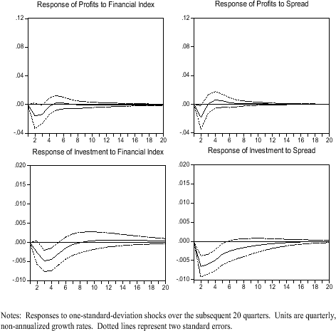
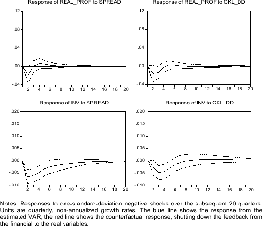
Figure 4 shows some of the results. The impulse-response functions reported in the figure demonstrate how the two real variables respond dynamically to one-standard-deviation shocks to the financial variables. (A one-standard-deviation shock to our financial index has a magnitude of 0.46. To put this magnitude in perspective, the magnitude of the change in the index during the 1988-1990 episode was about 2.5.) The short-run ordering of the shocks is assumed to be: (1) profits, (2) investment, (3) financial-health index, (4) credit spread. Both profits and investment respond negatively to adverse shocks to credit spreads and financial-institution condition. Over the two years following a shock to either financial variable, profits fall by a cumulative 2.7 percent, and investment falls by about 2 percent. The investment responses, in particular, are strongly statistically significant.

**Figure 4:** Impulse-Response Functions from Financial to Real Variables: Financial Index Ordered First
Figure 4 Data

**Figure 5:** Impulse-Response Functions from Financial to Real Variables: Credit Spread Ordered First
Figure 5 Data

These basic results are robust to a number of different specifications. Most importantly, since the reduced-form shocks to distance to default and credit spreads are highly correlated, the assumed structural ordering of these two shocks potentially makes a substantial difference in the extent to which importance is attributed to one over the other. However, even under the reverse ordering (Figure 5), which attributes all of the short-run correlation to exogenous changes in credit spreads, the effects of the financial-health shock still go in the same direction and are still significant, though less so. (The joint effect of the two financial shocks is insensitive to the ordering.)¹⁵

We also tried using consumption, rather than investment, in the VAR. Interestingly, we find similar, though quantitatively weaker, effects of changes in the health of financial intermediaries on consumption. This result is consistent with the idea that household credit, and thus spending, may also be affected by difficulties at financial institutions.

Returning to our baseline specification, shocks to the financial index account for about 12 percent of the long-run variance of investment and about 4 percent of the long-run variance in corporate profits. For comparison, shocks to credit spreads account for about 24 percent of investment variance and about 3 percent of profit variance. Looked at in another way, Figure 6 shows the specific effects of the shocks to the financial index on investment growth over our sample. This series is constructed as the difference between the actual investment-growth data and a counterfactual series generated by the VAR, with the financial-health shocks set to zero. (Equivalently, we could set all of the shocks other than those to the index to zero.) The figure shows that these shocks are responsible for swings of one to two percentage points in investment, on a quarterly basis, and that they have dragged investment down significantly during most recessions.

**Figure 6:** Effects of Financial-Health Shock on Investment Growth
Note. Shaded regions represent NBER recessions. Figure 6 Data

4.3 Effect of financial sector health in amplifying other shocks

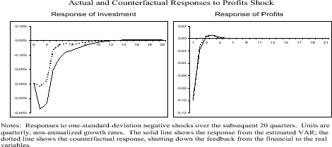
One can also examine how the financial variables contribute to the propagation of real shocks. To understand the importance of this propagation, we consider how an exogenous real shock (a shock originating in the non-financial sector) is amplified through the dynamic responses of the real and financial variables to each other. The blue lines in Figure 7 show the impulse-responses of investment and profits to a one-standard-deviation negative shock to profits in the VAR estimated above. The short-run effect on profit growth is strongly negative, although the series returns to normal within a couple of quarters. More importantly, investment growth slows by up to 0.5 percent following the shock and remains notably depressed for about two years. This result can be thought of as the outcome of two channels -- (1) the direct effect of profits on investment (operating, for example, through cash flow or expectations of lower future growth) and (2) the effect of tighter credit conditions that ensue when business conditions worsen. The second channel constitutes the amplification mechanism that interests us.

**Figure 7:** Actual and Counterfactual Responses to Profits Shock
Figure 7 Data

To isolate the effects of this mechanism, we recompute the impulse-response functions under the counterfactual assumption that the two financial variables have no effects on the two real variables (i.e., setting the eight corresponding coefficients in the VAR to zero). The red lines in Figure 7 show the outcome. Without the financial channels, the effect of the profits shock on investment growth is only about half of its previous magnitude and lasts only about half as long. Meanwhile, the effect of the profits shock on profits itself (i.e., the persistence of the shock) is largely unaffected when we shut down the effect from the financial variables. This result is consistent with the idea that the amplification mechanism operates like a credit constraint and works directly on investment with only minimal impact on the path of profits.

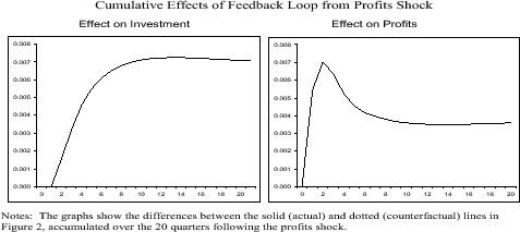
Figure 8 shows the cumulative effects of this channel on investment and profits. (This is constructed as the accumulated difference between the blue and red lines in Figure 7.) Over the five years following a one-standard deviation negative profits shock, we estimate that the financial amplification causes total investment and profits to be about 0.7 percent and 0.4 lower, respectively, than they otherwise would have been. To put these figures in perspective, the total cumulative responses to the shock after five years under the baseline model are 1.7 percent for investment and 10.4 percent for profits. Thus, the financial amplification accounts for about 40 percent of the investment response and about 4 percent of the profits response to an exogenous profits shock.

**Figure 8:** Cumulative Effects of Financial Amplification after a Shock to Profits
Figure 8 Data

5 Conclusion

Previous research, such as Mishkin (1991) and Bernanke (1983), has found that periods of financial crises are often followed by slower economic activity. In this paper, we provide a longer run perspective on the relationship of the health of the financial sector to economic activity, in particular on nonresidential investment. To do so, we construct a measure of financial sector health that includes periods of considerable stress, periods of notable strength, and moderate as well as severe fluctuations.

The results in this paper suggest that financial stability is connected to corporate investment, and that a deterioration in the health of the financial sector can act as a restraint on macroeconomic performance. We argue that one reason for this is that changes in financial institution health leads these institutions to tighten lending conditions and we find evidence consistent with this explanation. In addition, to a direct effect on investment, we also find that variations in the health of the financial sector also seem to amplify shocks to other parts of the economy.

Table 1
Tests for Granger Causality for lending standards and distance to default

Variable	Percent tightening standards: Coefficient	Percent tightening standards: Std. Error	Percent tightening standards: P-value	Change in distance to default: Coefficient	Change in distance to default: Std. Error	Change in distance to default: P-Value
standards lag1	0.801	0.124	6.45	0.005	0.006	0.74
standards lag2	0.080	0.117	0.68	-0.002	.006	-0.03
dist default lag1	-9.097	2.363	-3.85	0.121	0.121	0.99
dist default lag2	-0.916	2.562	-0.36	-0.021	0.132	-0.16
constant	0.413	1.088	0.38	-0.013	0.056	-0.23
Observations	70			70
	0.83			0.04

Granger causality (table 1)
For dist-default on standards: statistic	15.15
For dist-default on standards: Prob	0.001
For standards on dist-default: statistic	1.33
For standards on dist-default: Prob	0.514

Note: Standards are the net percent of banks reporting that they tightened lending standards and the distance to default measures is the change in the distance to default measure.

Table 2
Tests for Granger Causality for lending terms and distance to default

Variable	Percent tightening terms: Coefficient	Percent tightening terms: Std. Error	Percent tightening terms: P-value	Change in distance to default: Coefficient	Change in distance to default: Std. Error	Change in distance to default: P-Value
terms lag1	0.810	0.129	6.26	-0.001	0.004	-0.19
terms lag2	0.128	0.133	0.96	0.004	0.004	1.04
dist default lag1	-19.32	4.27	-4.52	0.038	0.127	0.30
dist default lag2	-4.28	4.55	-0.94	-0.098	0.135	-0.72
constant	-0.407	1.798	-0.23	0.029	0.053	0.55
Observations	70			70
	0.86			0.10

Granger causality (table 2)
For dist-default on terms: statistic	20.79
For dist-default on terms: Prob	0.000
For terms on dist-default: statistic	5.80
For terms on dist-default: Prob	0.055

Note: Lending terms are the net percent of banks reporting that they tightened lending terms and the distance to default measures is the change in the distance to default measure.

Bibliography

ASPACHS, O., C. GOODHART, D. TSOMOCOS, AND L. ZICCHINO (2007):

"Towards a Measure of Financial Stability," Annals of Finance.

BASURTO, M., C. GOODHART, AND B. HOFMANN (2006):

"Default, Credit Growth, and Asset Prices," IMF working paper number WP/06/223.

BAUDUCCO, S., A. BULIR, AND M. CIHAK (2008):

"Taylor Rule Under Financial Instability," IMF Working Paper WP/08/18.

BERNANKE, B. (1983):

"Nonmonetary Effects of the Financial Crisis in the Propagation of the Great Depression," American Economic Review, 73(3), 257-276.

BERNANKE, B., AND M. GERTLER (1989):

"Agency Costs, Net Worth, and Business Fluctuations," American Economic Review, 79(1), 14-31.

BERNANKE, B., M. GERTLER, AND S. GILCHRIST (1999):

"The Financial Accelerator in a Quantitative Business Cycle Framework," in Handbook of Macroeconomics, ed. by J. Taylor, and M. Woodford, vol. 1, pp. 1341-1393. Elsevier Science.

BLACK, F., AND M. SCHOLES (1973):

"The Pricing of Options and Corporate Liabilities," Journal of Poltical Economy, 81(3), 637-659.

CHAN-LAU, J., AND A. SY (2007):

"Distance-to-Default in Banking: A Bridge Too Far?," Journal of Banking Regulation, 9(1), 14-24.

CROSBIE, P., AND J. BOHN (2003):

Modeling Default RiskMoodys KMV Company.

FEDERAL DEPOSIT INSURANCE CORPORATION (1998):

Managing the Crisis: The FDIC and RTC Experience chap. 4: Continental Illinois National Bank and Trust Company, pp. 545-565. Washington DC, Federal Deposit Insurance Corporation.

FOSTER, D., AND D. NELSON (1996):

"Continuous Record Asymptotics for Rolling Sample Variance Estimators," Econometrica, 64(1), 139-74.

GIBSON, M. (1995):

"Can Bank Health Affect Investment? Evidence from Japan," Journal of Business, 68(3), 281-308.

GOODHART, C., P. SUNIRAND, AND D. TSOMOCOS (2005):

"A risk assessment model for Banks," Annals of Finance, 1, 197-224.

SMALL>3EM.5PT (2006):

"A time series analysis of financial fragility in the UK banking system," Annals of Finance, 2, 1-21.

GORTON, G., AND P. HE (2005):

"Bank Credit Cycles," NBER Working Paper Series No. 11363.

GROPP, R., J. VESALA, AND G. VULPES (2006):

"Equity and Bond Market Signals as Leading Indicators of Bank Fragility," Journal of Money, Credit, and Banking, 38(2), 399-428.

GUISO, L., A. KASHYAP, F. PANETTA, AND D. TERLIZZESE (2002):

"How Interest Sensitive is Investment? Very (when the data are well measured)," Mimeo.

HALDANE, A., S. HALL, AND S. PEZZINI (2007):

"A New Approach to Assessing Risks to Financial Stability," Bank of England Financial Stability Paper No.2.

HUBBARD, R. G., K. KUTTNER, AND D. PALIA (2002):

"Are There Bank Effects in Borrowers' Costs of Funds? Evidence from a Matched Sample of Borrowers and Banks," Journal of Business, 75(4), 559-581.

ILLING, M., AND Y. LIU (2003):

"An Index of Financial Market Stress for Canada," Bank of Canada Working Paper 2003-14.

LIU, Y., E. PAPAKIRYKOS, AND M. YUAN (2006):

"Market Valuation and Risk Assessment of Canadian Banks," Review of Applied Economics, 2(1), 63-80.

LOWN, C., D. MORGAN, AND S. ROHATGI (2000):

"Listening to Loan Officers: The Impact of Commercial Credit Standards on Lending and Output," Federal Reserve Bank of New York Policy Review, pp. 1-16.

MERTON, R. (1974):

"On the Pricing of Corporate Debt: The Risk Structure of Interst Rates," Journal of Finance, 29(2), 449-470.

MISHKIN, F. (1991):

"Asymmetric Information and Financial Crises: A Historical Perspective," in Financial Markets and Financial Crises, ed. by R. G. Hubbard, pp. 69-108. Chicago: University of Chicago Press.

PEEK, J., AND E. ROSENGREN (2000):

"Collateral Damange: Effects of the Japanese Bank Crisis on Real Activity in the United States," American Economic Review, 90(1), 30-45.

RAJAN, R. (1992):

"Insiders and Outsiders: The Choice Between Informed and Arm's Length Debt," Journal of Finance, 47(4), 1367-1400.

VON PETER, G. (2004):

"Asset Prices and Banking Distress: A Macroeconomic Approach," BIS Working Papers No. 167.

WOJNILOWER, A. (1980):

"The Central Role of Credit Crunches in Recent Financial History," Brookings Papers on Economic Activity, 1980(2), 277-326.

A. List of institutions

These institutions were among the largest 25 publicly traded financial institutions by assets in at least one quarter between 1973 and 2007.

American Express Co
Ameriprise Financial Inc
Associated First Capital
AXA Financial Inc
Bank of New England
Bank of New York Co
Bank One Corp
BankAmerica Corp
BankBoston Corp
Bankers Trust Corp
Barnett Banks Inc
BB&T Corp
Bear Stearns Companies Inc
C&S Sovran Corp (Citizens and Southern National)
Capital One Financial Corp
Chase Manhattan Corp
Chemical Bank
Citigroup
Continental Bank Corp
Corestates Financial Corp
Countrywide Financial Corporation
Eaton Vance Corp
Fifth Third Bancorp
Financial Federal Corp
First Boston Inc
First Chicago Corp
First City Bancorp
First Fidelity Bancorp
First Interstate Bancorp
First Investors Financial Services Group
First Pennsylvania Corp
First RepublicBank Corp
First Union
Firstar Corp
FleetBoston Financial Corp
Golden West Financial Corp
Goldman Sachs Group Inc
Great Western Financial
H. F. Ahmanson & Co
Hutton (E.F.) Group
Interfirst Corp
Irving Bank Corp
JPMorgan Chase & Co
Keycorp
Lehman Brothers Holdings Inc
Manufacturers Hanover Corp
Marine Midland Banks
Mayflower Bancorp Inc
MCorp
Mellon Financial Corp
Merrill Lynch & Co
Morgan Stanley
National City Corp
NationsBank
Norwest Corp
Paine Webber Group
PNC Financial Services Group Inc
Regions Financial Corp
Republic New York Corp
Security Pacific Corp
State Street Corp
Suntrust Banks Inc
Texas Commerce Bancshares
Travelers Group
US Bancorp
Wachovia Corp
Washington Mutual Inc
Wells Fargo & Co

Footnotes

* Email addresses: [email protected] , [email protected] [email protected]. The authors thank Mathias Drehmann as well as seminar participants at the Federal Reserve and the University of Groningen Center of International Banking, Insurance, and Finance for valuable comments. Kristen Payne provided excellent research assistance. The views presented in this paper are solely those of the authors and do not necessarily represent those of the Federal Reserve Board or its staff. Return to Text

1. Alternatively, some have argued that banks may choose to ease lending standards and hope that the higher returns on riskier loans will increase its profitability. Return to Text

2. While many of these arguments are focused on commercial banks, rising borrowing costs might also lead investment banks to charge more for underwriting equity or debt issuance and otherwise restrain their ability to provide intermediation services. Return to Text

3. We select these institutions by limiting our institutions to those with SIC codes between 6000 and 6300 or between 6700 and 6720. Government sponsored entities, such as Fannie Mae and Freddie Mac, are excluded from the sample. Return to Text

4. It is also possible to use the Foster-Nelson procedure to derive optimal flat-weight rolling variance estimators (i.e., fixed-length windows). However, as they show, this is generally not optimal. Importantly, our implementation imposes a constant conditional kurtosis of 3, consistent with conditional normality. Return to Text

5. One alternative measure is the average distance to default weighted by assets, which would weight concerns about the largest institutions more heavily. If the failure of a large financial institution matters more than the failure of a smaller one, this measure might be more appropriate. However, all of the institutions in our sample are already quite large. Further, if borrowers are able to substitute across financial institutions to some degree, then increases in the average distance to default owing to severe troubles at a single institution might suggest more significant problems in the financial sector than are actually the case. We show the weighted mean distance to default below. Return to Text

6. Still others have taken another approach to constructing indexes. Illing and Liu (2003) use a combination of banking sector, foreign exchange, equity market, and debt market variables to create stress index for Canada. Return to Text

7. The Herstatt bank failure is remembered for the issues related to clearing and settlement risk that arose. Herstatt had received some currency as part of a foreign exchange swap but the matching payments to the non-German banks had not yet been cleared. As a result, several banks lost considerable sums. Franklin National was the 20th largest bank in the U.S. at the time it failed. See Wojnilower (1980) for a discussion of these events. Return to Text

8. We exclude the day of the stock market crash from our estimates of volatility and distance to default. Return to Text

9. For further detail on the Continental Illinois episode see Federal Deposit Insurance Corporation (1998). Return to Text

10. Gropp, Vesala, and Vulpes (2006) provide further discussion of these and other other potential biases. Return to Text

11. Respondents are also asked about changes in standards and terms to business customers of other sizes and to their residential and consumer loan customers. We focus here on the large business borrowers. Return to Text

12. Our estimation procedure is similar to Aspachs, Goodhart, Tsomocos, and Zicchino (2007). They look at the impact on inflation and GDP growth of a probability of default measure, derived from a distance to default measure, for the banking sector and a measure of bank profitability. Their probability of default index is transformed so that it takes on values greater than zero when it exceeds a particular threshold and is zero otherwise. Our measure uses a distance to default measure without transforming it into a probability of default.
There is a complementary, but different, line of research that explores the relation of the real and financial sectors but focuses largely on how the shocks to the real economy might affect the financial sector. See, for example, Haldane, Hall, and Pezzini (2007). Return to Text

13. We also ran a specification using S&P 500 equity returns, in addition to credit spreads, to control for market conditions, with largely the same results, although the assumed structural ordering makes a bigger difference in this case. Return to Text

14. The results are also robust to a shorter sample that includes only post-Great Moderation data. Return to Text

15. To guard against potential omitted-variable bias and unmodeled expectations we tried estimating several larger VAR systems. In particular, we experimented with including GDP, unemployment, and labor productivity as additional real variables. We also included short- and long-term interest rates and inflation to allow for monetary-policy channels. In all cases, our estimates remained significant and qualitatively similar. Return to Text

^♣ This version is optimized for use by screen readers. Descriptions for all mathematical expressions are provided in LaTex format. A printable pdf version is available. Return to Text