FEDS Notes
July 19, 2024
Has the Inflation Process Become More Persistent? Evidence from the Major Advanced Economies
Andrea De Michelis, Grace Lofstrom, Mike McHenry, Musa Orak, Albert Queralto, Mikaël Scaramucci1
The sustained surge in inflation around the world following the pandemic has raised the possibility that the inflation process has become more persistent. Such a rise in persistence could result from firms and households putting greater weight on past inflation outcomes in their price- and wage-setting decisions than they did in the recent past, say, because they have less conviction that inflation will return promptly to target. Greater persistence would, in turn, complicate central banks' task of bringing inflation back to target. Against the background of the recent slowdown in the disinflation process, this note reviews inflation dynamics across selected major advanced economies and finds that the inflation process has indeed become more inertial in the period following the COVID-19 pandemic, even after shocks to energy prices and supply disruptions are controlled for. We then use a canonical new-Keynesian model estimated using data from the euro area—which remains particularly vulnerable to energy price increases, and where the disinflation process has slowed this year—to show that higher inflation persistence would call for a significantly tighter monetary policy stance in response to renewed adverse supply shocks.
Empirical framework: a Phillips curve for core inflation
Our empirical strategy is to examine the inflation process using a backward-looking Phillips curve, an equation commonly used to relate core inflation to resource slack dating back to Phillips (1958). Specifically, we assume that core inflation evolves according to
$$\pi_t=\alpha+\gamma_1 \pi_{t-1}+\gamma_2 \pi_{t-2}+\lambda x_t+\beta s_t + \delta e_t +\varepsilon_t\ (1)$$
where $$\pi_t$$ is core inflation in quarter $$t$$, $$x_t$$ is the output gap, $$e_t$$ is (lags of) energy price inflation, $$s_t$$ is an index measuring global supply chain disruptions, and $$\varepsilon_t$$ is an uncorrelated error term.2 We estimate equation (1) by OLS separately for Canada, the euro area, Japan, the U.K., and the U.S. using quarterly data since 2000. It is worth highlighting that this specification of the Phillips curve does not explicitly control for inflation expectations. Still, to the extent that agents form expectations based on realized inflation outcomes, inflation expectations should be captured by the coefficients on lagged inflation. In addition, because standard measures of longer-run inflation expectations—such as 5- and 10-year-ahead inflation forecasts by Consensus Economics—tend to be very stable, inflation expectations are subsumed to some degree in the constant.
This note focuses on the post-pandemic changes in the persistence coefficients, while much of the recent literature has instead focused on the changes in the slope of the Philips curve.3 To determine whether persistence has increased, we examine the sum of the coefficients on lagged core inflation, $$γ_1$$ and $$γ_2$$.4 This sum measures the degree of inertia in the inflation process, with values close to 0 indicating that above-target inflation would not be much of a signal for future inflation and values close to 1 indicating that elevated inflation would persist for some time, even in the absence of further inflationary shocks.5 In line with the findings of Bernanke and Blanchard (2024) that the unusual size and persistence of both energy price changes and supply disruptions have been important drivers of the recent surge and of the stickiness of inflation across many advanced economies, our specification of the Phillips curve explicitly controls for these factors. Accordingly, our methodology is designed to yield a clear and simple picture of whether the inherent dynamics of the inflation process have changed after accounting for the persistence of the recent large shocks.
We find that inflation persistence has broadly risen after the pandemic. As shown in figure 1, for the five selected economies, the sum of the lag coefficients including the post-pandemic period (the red bars) is above the values estimated just over the pre-pandemic period (the blue bars).6 Even though the rise in persistence is not always statistically significant at the country level, we take signal from the fact that the point estimates have increased for all economies, and the differences in the point estimates appear economically important.

Note: Pre-pandemic sample period is from 2000:Q1 to 2019:Q4, while sample including post-pandemic data is from 2004:Q1 to 2023:Q4. Key identifies in order from left to right.
Source: Haver Analytics; Authors' calculations.
To explicitly test if this cross-country evidence is indicative of a statistically meaningful change, we perform a panel regression analysis that benefits from both cross-sectional and time-series variations. We continue to assume that core inflation evolves according to equation (1), but we estimate the equation with panel data (thus imposing that the coefficients are the same across countries) and augment our specification with a set of interaction terms between the lags of core inflation and a dummy for the post-pandemic period to isolate the effects of post-pandemic inflationary dynamics on persistence. Specifically, we estimate the following equation:
$$\pi_{i,t}=\alpha+\gamma_1 \pi_{i,t-1}+\gamma_2 \pi_{i,t-2}+\eta_1 \pi_{i,t-1} \times D_{t\geq 2021:Q1}+\eta_2 \pi_{i,t-2} \times D_{t\geq 2021:Q1}+ \lambda x_{i,t}+\beta s_{i,t} + \delta e_{i,t} +\varepsilon_{i,t}\ (2)$$
Where $$D_{t\geq 2021:Q1}$$ is a dummy variable that is equal to 0 prior to 2021:Q1 and to 1 from 2021:Q1 onward.7
The sum of the two interaction terms captures the average change in persistence across the economies in the post-pandemic period relative to the pre-pandemic period. As shown in table 1, we find that the post-pandemic increase in persistence is statistically significant. The magnitude of the increase is also economically significant, with the estimated persistence roughly doubling from about 0.3 in the pre-pandemic period to about 0.6 in the sample including the post-pandemic period. All told, the cross-country evidence suggests that there has been a statistically significant and economically large increase in inflation persistence.8
Table 1: Persistence Estimates from Cross-Country Panel Data
| Point estimate | Lower bound | Upper bound | |
|---|---|---|---|
| Pre-pandemic persistence | 0.33*** | 0.26 | 0.4 |
| Post-pandemic increase in persistence | 0.31*** | 0.25 | 0.37 |
*** Significant at the 1 percent level.
Note: Change in persistence refers to the sum of the coefficients on a set of interaction terms between the lags of core inflation and the dummy for the post-pandemic period, which begins in 2021:Q1.
Source: Haver Analytics; Authors' calculations.
Case study: Implications of higher inflation persistence in the euro area
To illustrate the consequences of a more-persistent inflation process, we use a standard New Keynesian general equilibrium model estimated using euro-area data. We use the model to simulate supply, demand, and monetary policy shocks that exactly replicate euro-area GDP growth, core inflation, and the policy rate through the first quarter of 2024, assuming a moderate amount of inflation persistence.9 As shown in figure 2, we find that a combination of adverse supply shocks and positive demand shocks accounts for the bulk of the increase in inflation between early 2021 and late 2022, with roles for demand and supply shocks of similar magnitude, and with a positive but smaller role for expansionary monetary shocks. This decomposition is informed by the evolution of GDP growth, which has underperformed relative to the model's projection absent post-2021 shocks (labelled "initial conditions" and shown by the gray bars), but which would have underperformed even more if only supply shocks had occurred.10 Absent shocks, the model implies a relatively fast decline in inflation toward 2 percent and a steep policy easing (blue dashed lines in figure 3).
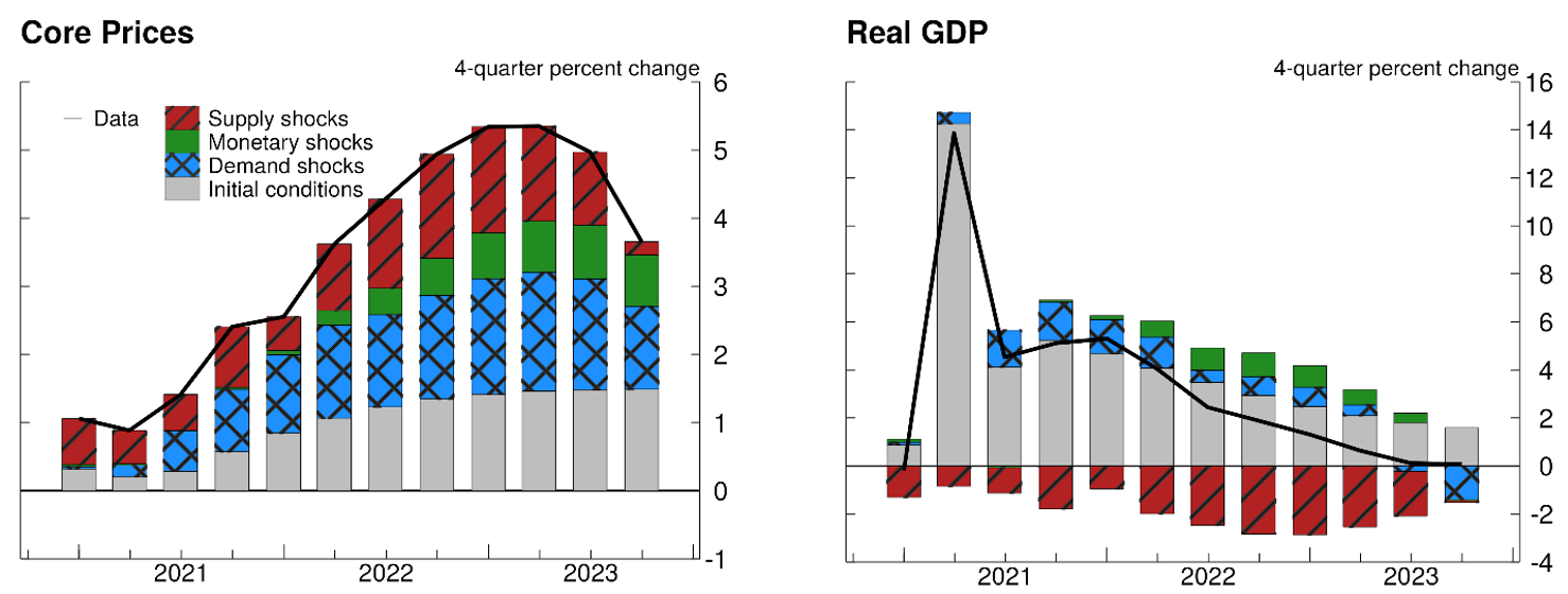
Note: The red, green, and blue bars show the contributions of the post-2021 supply, monetary, and demand shocks, respectively. The grey bars show the contribution of initial conditions, reflecting shocks occurring before 2021:q1 and other long-run factors like trend growth (the model is estimated on demeaned GDP growth data).
Source: Authors' calculations
Figure 3. Implications of Higher Inflation Persistence for the Transmission of Supply Shocks in the Euro Area
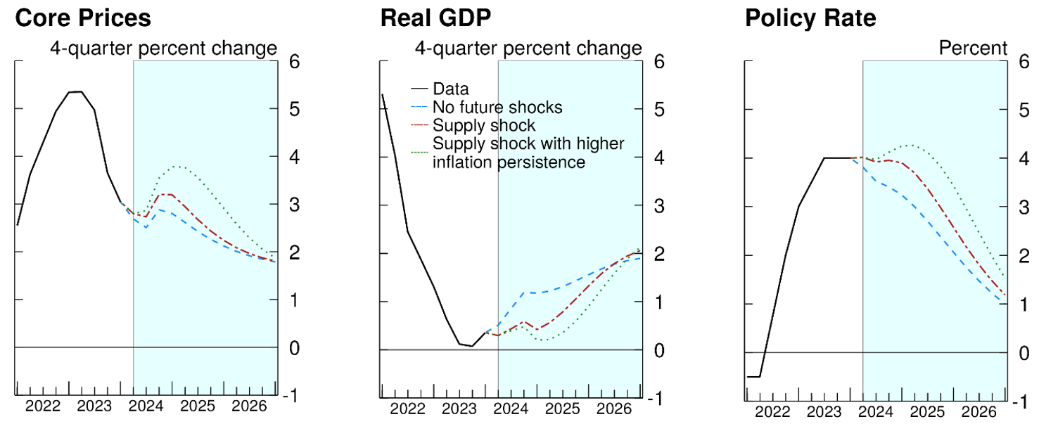
Source: Authors' calculations
We first envision an alternative scenario in which the euro area faces an additional adverse supply shock—for example, due to a further run-up in energy prices or renewed adverse pressures on global supply chains. We assume the shock occurs in the second quarter of 2024 and size it to a unit of its estimated standard deviation—capturing a shock of typical size, as opposed to the unusually large adverse supply shocks hitting the euro area over 2021 and 2022, which exceeded 2 standard deviations in some quarters. As seen in the red dash-dotted lines in figure 3, inflation runs somewhat higher than in the no-shock case, but the shock is not large enough to call for an increase in the policy rate from its current level.
We then contrast this case with another in which the inflation process in the euro area becomes more persistent, to the degree implied by our empirical analysis. Motivated by this year's slower disinflation, we assume that this change occurs in 2024. We model this higher persistence as arising from a shift in behavior whereby firms and workers place more weight on recently observed levels of inflation and less weight on the 2 percent inflation target when setting prices and wages, consistent with inflation expectations being less well anchored around the target. We then simulate the model-predicted paths under this higher persistence, shown by the green dotted lines, again assuming a negative supply shock in the second quarter of 2024.
The consequences of the supply shock are considerably more adverse with higher inflation persistence. Inflation reaches 3.75 percent in 2025, almost 1 percentage point higher than if the same shock had occurred with lower inflation persistence. The policy rate increases relative to its current level and remains higher for longer. Specifically, the policy rate is around 3.75 percent by end-2025, almost 1 percentage point higher than if the same shock had occurred absent the increase in persistence. The higher policy rate path needed to rein in inflation weakens aggregate demand, bringing GDP growth to almost zero in 2025.
In conclusion, the findings of this note suggest that central banks should factor in the possibility of a more inertial inflation process and thus consider maintaining a restrictive policy for longer to fully extinguish the past inflationary shocks.
References:
Alp, Harun, Matthew Klepacz, and Akhil Saxena (2023). "Second-Round Effects of Oil Prices on Inflation in the Advanced Foreign Economies," FEDS Notes. Washington: Board of Governors of the Federal Reserve System, December 15, 2023.
Benigno, Pierpaolo & Gauti B. Eggertsson (2023). "It's Baaack: The Surge in Inflation in the 2020s and the Return of the Non-Linear Phillips Curve (PDF)," NBER Working Papers 31197, National Bureau of Economic Research, Inc.
Bernanke, Ben and Olivier J. Blanchard (2024). "An Analysis of Pandemic-Era Inflation in 11 Economies," PIIE Working Paper 24-11 (Washington: Peterson Institute for International Economics, May), https://www.piie.com/sites/default/files/2024-05/wp24-11.pdf.
Federal Reserve Bank of New York, Global Supply Chain Pressure Index.
Furlanetto, Francesco, and Antoine Lepetit (2024). "The Slope of the Phillips Curve," Finance and Economics Discussion Series 2024-043. Washington: Board of Governors of the Federal Reserve System.
O'Trakoun, John (2023). "Inflation Staying Persistent," Federal Reserve Bank of Richmond, May 2023.
Phillips, A.W. (1958). "The Relation between Unemployment and the Rate of Change of Money Wage Rates in the United Kingdom, 1861-1957," Economica, 25:283-99, https://doi.org/10.1111/j.1468-0335.1958.tb00003.x.
1. The views expressed in this note are solely the responsibility of the authors and should not be interpreted as reflecting the views of the Board of Governors of the Federal Reserve System or of anyone else associated with the Federal Reserve System. We thank William Wu for excellent research assistance. We are also thankful to Shaghil Ahmed, Deepa Datta, Etienne Gagnon, Ekaterina Paneva, and Jeremy Rudd for valuable feedback. All errors and omissions are responsibility of the authors. Return to text
2. We are using PCE inflation for the U.S. and CPI inflation for all other economies.
Energy prices are measured as the quarterly percent change in the energy component of the relevant price index—a comprehensive measure encompassing all types of energy products consumed by households that is inclusive of government levies, refinery margins, and marketing costs. The equation includes four lags of energy price inflation— that is, $$\delta e_t$$ stands for $$\Sigma_{i=1}^{4}\delta_i e_{t-1}$$—to control for the long delays through which energy prices may affect core prices. The fact that we do not include any contemporaneous measures of energy prices is consistent with the findings of Alp, Klepacz, and Saxena (2023), who show that it takes some time for changes in retail energy prices to pass through to core prices.
Supply chain disruptions are measured using the Global Supply Chain Pressure Index (GSCPI) index of Federal Reserve Bank of New York.
Equation (1) also includes dummy variables for 2020:Q1, 2020:Q2, 2020:Q3, and 2020:Q4 to control for the mismeasurement of certain independent variables, especially the output gap, during the onset of the pandemic. Return to text
3. For studies focusing on post-pandemic changes in the slope coefficient, see Benigno and Eggertson (2023) and Furlanetto and Lepetit (2024). One study that also focuses on changes in inflation persistence is O'Trakoun (2023). Using an AR1 model on quarterly U.S. core PCE inflation, O'Trakoun finds that persistence more than doubled since its pre-pandemic average. Return to text
4. We test the joint significance of up to four lags of core inflation to choose the optimal number of lags for each country-level regression and conclude that including more than two lags of core inflation does not significantly improve our estimates. Return to text
5. In the case of the sum equaling unity, the equation above turns into a pure "accelerationist" Phillips curve, where a persistently positive output gap leads to ever-rising inflation. Return to text
6. The rise in persistence when the post-pandemic period is included would be even larger if we did not control for energy prices and supply disruptions, with energy prices playing a larger role in Europe and supply disruptions playing a larger role in Canada and the United States. These findings suggest that our methodology can reasonably account for the influence of the persistence of these shocks, helping to avoid overestimating the inherent persistence of the inflation process. Return to text
7. The panel regression also includes country fixed effects. Return to text
8. The panel results are robust to several changes to the specification of the cross-country analysis. In particular, we evaluated two alternative specifications of equation (2): (i) one that allowed country-specific persistence coefficients for the pre-pandemic period and (ii) one that continued to assume common pre-pandemic persistence coefficients while allowing country-specific interaction dummies. For these alternative specifications, we continued to find rises in persistence in the post-pandemic period that are similar in magnitude and significance to the baseline results reported in table 1. Return to text
9. Demand shocks capture shifts in spending caused by household and business confidence, financial constraints, and factors other than monetary policy driving aggregate demand. Supply shocks capture disruptions in the supply of nonlabor production inputs, such as energy and imported intermediate inputs. Monetary policy shocks capture deviations of the policy rate from the estimated monetary policy rule. Because we use three types of shocks for three time series, we recover a unique time path for each shock. Return to text
10. Initial conditions are computed by simulating the model from the last quarter of 2020 onwards, assuming that no shocks occur after that quarter. Thus, initial conditions capture the effects of shocks that occurred prior to 2021:Q1 as well as other long-run factors, such as the central bank's inflation target and the trend rate of GDP growth (the model is estimated on demeaned GDP growth data). Return to text
de Michelis, Andrea, Grace Lofstrom, Mike McHenry, Musa Orak, Albert Queralto, and Mikaël Scaramucci (2024). "Has the Inflation Process Become More Persistent? Evidence from the Major Advanced Economies," FEDS Notes. Washington: Board of Governors of the Federal Reserve System, July 19, 2024, https://doi.org/10.17016/2380-7172.3562.
Disclaimer: FEDS Notes are articles in which Board staff offer their own views and present analysis on a range of topics in economics and finance. These articles are shorter and less technically oriented than FEDS Working Papers and IFDP papers.