FEDS Notes
June 28, 2024
Lessons from the Co-movement of Inflation around the World
Danilo Cascaldi-Garcia, Luca Guerrieri, Matteo Iacoviello, and Michele Modugno1
The aftermath of the COVID-19 pandemic saw a surge in inflation around the world, reflecting rapid increases in the demand for goods, strained supply chains, tight labor markets, and sharp hikes in commodity prices exacerbated by the Russian war on Ukraine. As illustrated in figure 1, this inflation surge was synchronized across advanced and emerging economies, not only for total inflation but also for its core component. The left panel of the figure highlights co-movement in total (headline) inflation, largely driven by globally determined food and energy prices. Beyond those usual suspects, the right panel shows substantial co-movement for core inflation, which abstracts from changes in food and energy prices.
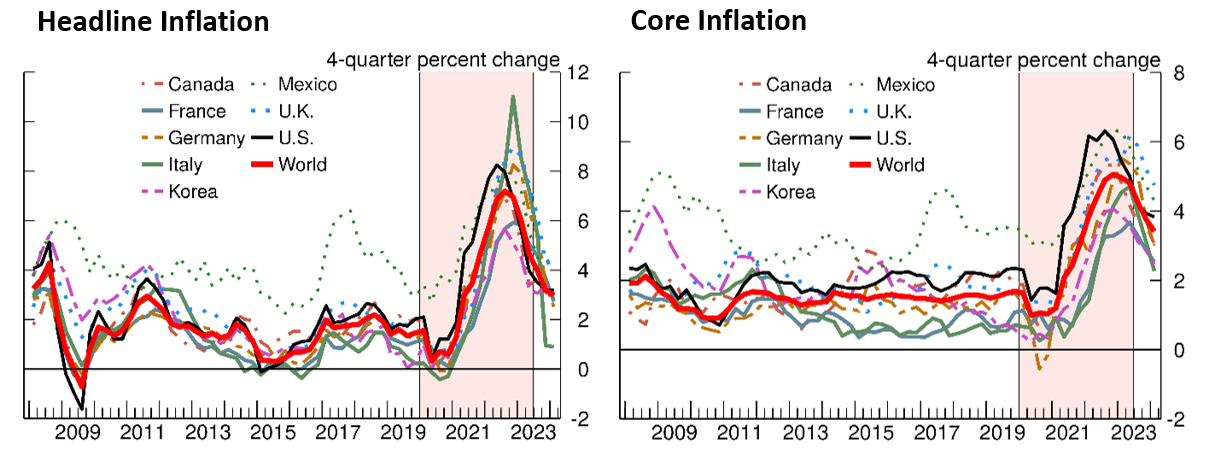
Note: Inflation series are 4-quarter percent changes of consumer price indexes, and world inflation is GDP-weighted 4-quarter percent change of consumer price indexes for selected economies. Data extend through 2024:Q1. Shaded area refers to period in which the World Health Organization declared COVID-19 a public health emergency. World inflation, the red line, is a GDP-weighted average of the inflation measures for 26 economies.
Source: National sources via Haver Analytics; FRB staff calculations; World Health Organization.
A host of factors can explain the global co-movement in headline and core inflation. First, fluctuations in global food and energy prices can influence the production costs of all firms and feed through to country-specific prices. But there are other possible explanations, including global shocks, global supply constraints, as well as synchronous policy responses. In this note, we weigh these explanations against each other using a statistical model.
Our statistical model allows a quantification of the degree of inflation synchronicity across historical episodes and of how the recent co-movement could influence inflation going forward. In the model, estimated with data starting in the early 1960s, world inflation is decomposed into a global component—capturing cyclical co-movement in inflation across economies—and country-specific components. The model includes distinct global components for noncore (food and energy) and core inflation, which facilitates linking their changes to a host of economic drivers.
Our main finding is that the global component of inflation accounts for a large part of the variation in world inflation, including during the notable inflationary episodes of the energy crises of the 1970s and the 1980s, as well as the post-COVID period. Of note, we find that the recent rise in global inflation is linked to both commodity-driven shocks and to global activity shocks—such as the sharp decline and rebound in activity due to the COVID-19 pandemic and the associated labor market shortages.
The Model
We use a dynamic factor model (DFM) to extract the common components of sectoral inflation measures across countries. Inflation is disaggregated into core and noncore sectoral measures.2 Formally, the observation equation of the DFM is
$$$$ \pi_{ist} = \chi_{ist} + c_{ist} + \xi_{ist} \ \ \ \ \ \ \ \xi_{ist} \sim N(0,R_{i,i}^{s})\ i.i.d. ,$$$$
where $$\pi_{ist}$$ is the inflation rate for country $$ i $$ in sector $$ s $$ (core, noncore) at time $$ t $$, and $$ \chi_{ist} $$ is the common component. The terms $$ c_{ist} $$ and $$\xi_{ist} $$ are a time-varying constant and white noise, respectively.3 In turn, the common component, $$\chi_{ist}$$, is defined as
$$$$\chi_{ist} = \lambda_{is0} f_{st} + \lambda_{is1} f_{st-1} , $$$$
where $$ f_{st} $$ is the common factor for sector s, invariant across countries, and $$ \lambda_{is0} $$ is a factor loading specific to each country and sector. The evolution of the unobserved, sector-specific factors follows the transition equation
$$ f_{st} = a_{s1} f_{st-1} + a_{s2} f_{st-2} + a_{r1} f_{rt-1} + a_{r2} f_{rt-2} + u_{st}, $$ where $$ u_{st} \sim N(0,Q_{ss})\ i.i.d. $$
The coefficients $$ a_{s1} $$ and $$ a_{s2} $$ capture the persistence of the sector-specific factor. When $$ s $$ in the transition equation above refers to the core sector, the $$ r $$ in the term $$ a_{r1} f_{rt-1} + a_{r2} f_{rt-2} $$ refers to the noncore sector, and vice-versa. This specification allows us to capture the passthrough of noncore inflation to core inflation or, conversely, the passthrough of core inflation to noncore inflation. Finally, the term $$ u_{st} $$ is a white noise process.
For estimation purposes, the inflation term $$ \pi_{ist} $$ is calculated as the 4-quarter percent change in the consumer price index (core and non-core) or its local equivalent. We use data for 26 economies, including the U.S., representing about 60 percent of world GDP.4 The estimation sample runs from 1961:Q1 through 2024:Q1.5 We impose a sample break in 1994:Q4 to capture the change in volatility of inflation after the Great Moderation. We estimate the parameters by maximum likelihood, following the method in Bańbura and Modugno (2014) for state-space models using an unbalanced panel.
Finally, the global components of core and noncore inflation are defined as the GDP-weighted sums of the common components for each country. Accordingly,
$$$$ \chi_{st} = \sum_{i} w_{it} \chi_{ist}, $$$$
where the weights for each economy, $$ w_{it} $$, are shares of GDP at purchasing power parity.6
Estimation Results
Figure 2 shows world headline inflation and our estimate of its global component, as well as the estimates for the global components of core and noncore inflation separately.7 The global component of headline inflation was high and volatile in the 1970s and 1980s, moderated in the 1990s and 2000s, and surged again starting in 2021, pushed up by both core and noncore components (left panel).
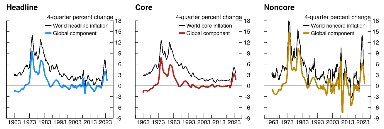
Note: World inflation is the GDP-weighted, 4-quarter percent change of consumer price indexes for selected economies. Global components are GDP-weighted aggregates of each economy's common component. Noncore inflation encompasses food and energy categories. Headline inflation is the aggregate of core and noncore inflation using economy-specific weights.
Source: National sources via Haver Analytics; FRB staff calculations.
Between the 1960s and the mid-1990s, world core inflation was also high and volatile, and its global component accounted for much of its volatility (middle panel). By contrast, from the mid-1990s until 2020, world core inflation was low, with the global component contributing little to its movement. Beginning in 2021, however, world core inflation rose remarkably, and it did so with a high degree of co-movement across economies, as evidenced by the sharp jump in its global component.
World noncore inflation is substantially more volatile than world core inflation (right panel). Its behavior across the entire sample closely tracks the global component, reflecting limited local variation beyond the influence of global commodity markets for food and energy prices.
Table 1 reports the contribution of the global components to the variation in inflation. On average, the global components account for a large share of the variation in inflation in different time periods. The share is consistently high for headline inflation, reflecting the importance of the global component for noncore inflation. By contrast, there are greater differences across periods in the share of core inflation accounted by the global component.
Table 1: Inflation Variation Explained by the Global Component
(Percent of total share)
| 1961–94 | 1995–2019 | 2020-2024:Q1 | |
|---|---|---|---|
| Headline inflation | 88 | 74 | 98 |
| Core inflation | 86 | 54 | 92 |
| Noncore inflation | 80 | 74 | 59 |
Note: Share of inflation explained by co-movement is calculated as the R2 of a regression of each economy's cyclical inflation on common factors for core and noncore inflation. Cyclical inflation is each economy's 4-quarter inflation subtracted from its estimated trend. Indicator is the GDP-weighted mean of the R2 for each economy.
Source: National sources via Haver Analytics; FRB staff calculations.
The global components of inflation also have some predictive power for the near-term path of inflation. Historically, the global components have been persistent; once they start moving, they stay the course and take some time to reverse. This persistence, coupled with the fact that the global components of core and noncore inflation have started to decline, suggests the world disinflation process will continue (figure 3). This process is consistent with a scenario of a gradual return of inflation toward central-bank targets amid a slow and gradual resolution of supply-chain disruptions and ongoing resolution of labor-market imbalances.8
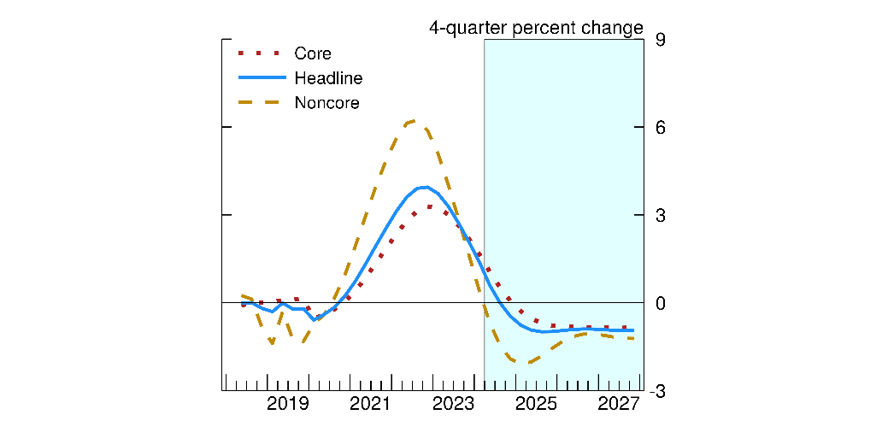
Note: Global components are GDP-weighted components estimated through a factor model that isolates co-movement from economy-specific trends and transitory movements. Noncore inflation encompasses food and energy categories. Forecast shown is derived from the factor model and driven by the statistical persistence of the global components. Headline global component is the weighted average of core and noncore global components using economy-specific weights.
Source: National sources via Haver Analytics; FRB staff calculations.
Disentangling the Economic Drivers
So far, we have focused on the global components of inflation using a model that abstracts from the identification of their economic drivers. Isolating these drivers is complicated by the fact that core and noncore inflation are not independent of each other, as they both respond to and interact with global economic developments. Accordingly, we estimate a vector autoregressive (VAR) model that can account for these interactions and parse out the drivers of inflation.
The VAR model includes quarterly observations on the global components of core and noncore inflation, an index of nonfuel commodity prices, crude oil prices, global GDP, and an index of shortages in the labor market.9 These variables capture a broad array of underlying supply and demand forces that influence world inflation. We estimate the VAR model with four lags with Bayesian methods using a standard Minnesota prior. Consistent with the approach for the DFM, we split the estimation sample into two sub-periods (1961:Q1 to 1994:Q4 and 1995:Q1 to 2024:Q1) to account for structural changes in inflation.
The identification of the VAR is based on a recursive scheme in which the variables are ordered as follows: global GDP, shortages, global component of core inflation, oil prices, commodity prices, global component of noncore inflation. We label the combined innovations to the first three variables global activity shocks and the combined innovations to the last three variables commodity shocks. According to this identification scheme, global activity shocks affect the global components of both core and noncore inflation within the quarter. Commodity shocks also affect the global component of noncore inflation contemporaneously but only affect the global component of core inflation with a lag. By construction, the combined shocks in the VAR fully account for the movements in the global component of headline inflation. Accordingly, any gap between world headline inflation and its global component can be attributed to idiosyncratic, country-specific shocks that are left out of the VAR model.
We use the model to shed light on the relative prominence of the two groups of shocks across global inflation cycles. Figure 4 illustrates the results of this exercise. In the 1970s and 1980s, commodity shocks were the primary force driving the rise and fall in world headline inflation (left panel). The more recent inflation episode is strikingly different and results from the combination of both groups of shocks (right panel). Commodity shocks drove part of the rise in world inflation, but global activity shocks—such as the sharp decline and rebound in activity due to the COVID-19 pandemic as well as the associated labor market shortages—also played an important role. Additionally, idiosyncratic shocks were drivers of the surge in global inflation in 2022 and its decline in 2023. These shocks may capture economy-specific forces, including natural gas disruptions that more greatly affected European economies in the aftermath of Russia's war on Ukraine.
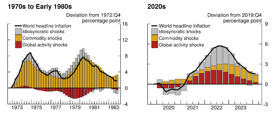
Note: Figure 4 illustrates decomposition for selected inflationary periods stemming from vector autoregressive models estimated from 1961:Q1 to 1994:Q4 (left panel) and from 1995:Q1 to 2024:Q1 (right panel). Global component of headline inflation and its decomposition are constructed from economy-specific core inflation weights and aggregated with GDP weights. Global activity shocks combine shocks to the global component of core inflation, to global GDP, and to labor market shortages. Commodity shocks combine shocks to the global component of noncore inflation, to oil prices, and to global commodity prices. Noncore inflation encompasses food and energy categories.
Source: National sources via Haver Analytics; FRB staff calculations.
In sum, through the lens of the model, the ongoing disinflation is driven by waning effects of commodity price shocks and by a gradual normalization of global activity amid the resolution of shortages and of imbalances in labor markets.
References
Akinci, O., Benigno, B., Cesar Heymann, R., di Giovanni, J., Groen, J., Lin, L., and Noble, A. (2022), "The Global Supply Side of Inflationary Pressures," Federal Reserve Bank of New York, Liberty Street Economics (blog), January 28.
Bai, X., Fernández-Villaverde, J., Li, Y., and Zanetti, F., (2024), "The Causal Effects of Global Supply Chain Disruptions on Macroeconomic Outcomes: Evidence and Theory," NBER Working Paper Series 32098 (Cambridge, Mass.: National Bureau of Economic Research, February).
Bańbura, M. and M. Modugno (2014)," Maximum likelihood estimation of factor models on data sets with arbitrary pattern of missing data," Journal of Applied Econometrics, 29: 133-160.
Caldara, D., M. Iacoviello, and D. Yu (2024), "Measuring Shortages Since 1900," Mimeo, Federal Reserve Board, https://www.matteoiacoviello.com/research_files/SHORTAGE_PAPER.pdf.
Cascaldi-Garcia, D., Luciani, M., and Modugno, M. (2023), "Lessons from Nowcasting GDP across the World," International Finance Discussion Papers 1385 (Washington: Board of Governors of the Federal Reserve System, December).
1. We thank our colleagues at the Federal Reserve Board for comments on an earlier draft. Kellen Lynch and Chris Machol provided excellent research assistance. The views expressed in this note are solely the responsibility of the authors and should not be interpreted as reflecting the views of the Board of Governors of the Federal Reserve System or of anyone else associated with the Federal Reserve System. Return to text
2. Dynamic factor models have been widely used as an efficient way of extracting meaningful economic signals from large sets of unstructured data. Their applications range from data summary and dimension reduction to accurately forecasting the economy. See Cascaldi-Garcia, Luciani, and Modugno (2023) for a review of the method. Return to text
3. The time-varying constant is modelled as a driftless random walk. Return to text
4. The economies covered are Australia, Austria, Belgium, Canada, Denmark, Finland, France, Germany, Ireland, Israel, Italy, Japan, Korea, Mexico, the Netherlands, New Zealand, Norway, Portugal, Singapore, Spain, Sweden, Switzerland, Taiwan, Thailand, the U.K., and the U.S. Data are from official national sources via Haver Analytics. Return to text
5. Not all the inflation series for the 26 economies in our dynamic factor model extend all the way back to 1961:Q1, the start of our estimation sample. In particular, both core a noncore inflation data are available from 1961:Q1 for Finland, Italy, Japan, Switzerland, and the U.S., from 1961:Q2 for the Netherlands, and from 1962:Q1 for all the other countries in our sample. Return to text
6. We apply analogous weights to construct overall measures of world inflation and its trend. Return to text
7. The global component is expressed in deviation from the world inflation's time-varying long-run trend. Return to text
8. A similar point on the supply disruption forces driving inflation is made by, among others, Akinci, Benigno, Cesar Heymann, di Giovanni, Groen, Lin, and Noble (2022); and Bai, Fernández-Villaverde, Li, and Zanetti (2024). Return to text
9. The global components of core and noncore inflation are estimates from the factor model and are displayed in figure 2 (middle and right panels). Global GDP is constructed using data from Haver Analytics and authors' calculations (four-quarter percent change). The commodity price index is the Reuters–CRB Spot Commodity Price Index for raw industrials and foodstuffs (in logs). The oil price index is Crude Oil Prices: West Texas Intermediate (in logs). The shortage measure is a news-based indicator of shortages of foods, labor, and industrial goods constructed and described in Caldara, Iacoviello, and Yu (2024). Return to text
Cascaldi-Garcia. Danilo, Luca Guerrieri, Matteo Iacoviello, and Michele Modugno (2024). "Lessons from the co-movement of inflation around the world," FEDS Notes. Washington: Board of Governors of the Federal Reserve System, June 28, 2024, https://doi.org/10.17016/2380-7172.3543.
Disclaimer: FEDS Notes are articles in which Board staff offer their own views and present analysis on a range of topics in economics and finance. These articles are shorter and less technically oriented than FEDS Working Papers and IFDP papers.