FEDS Notes
May 24, 2024
Measuring Bank Credit Supply Shocks Using the Senior Loan Officer Survey
Michele Cavallo, Juan Morelli, Rebecca Zarutskie, Solveig Baylor1
Estimating the effects that bank credit supply has on macroeconomic activity has long been an area of active research.2 A key challenge in pursuing this goal is the ability to measure such shocks to banks' supply of credit separately from shocks to borrowers' demand for credit.
In this note, we present a measure of credit supply shocks that exploits bank-level responses to the Federal Reserve's Senior Loan Officer Opinion Survey on Bank Lending Practices (SLOOS) applying a variation of the methodology introduced by Bassett et al. (2014), which consists of purging banks' responses regarding changes in lending standards from the influence of macroeconomic, financial, and bank-specific factors. Building on such methodology, we extend the analysis along four lines. First, we consider a different set of bank-specific factors with the aim of better capturing innovations that could affect banks' reported changes in standards with delay. Second, we consider a longer sample period, which allows us to assess the changes in the supply of bank credit implied by the developments in the banking sector over the last couple of years. Third, based on the regression analysis, we provide a decomposition of banks' changes in standards into the contributions made by the various explanatory factors. Fourth, we construct measures of bank credit supply shocks that are specific to the major SLOOS loan categories.
Our estimates show that in the second half of 2022 and the first quarter of 2023 there was a sizable negative bank credit supply shock, as banks restricted credit supply in excess of what would have been expected given the historical empirical relationship between past bank lending standards, determinants of borrower demand, banks' characteristics, and changes in the macroeconomic outlook. In contrast, over the remainder of 2023, our measure does not point to the presence of further adverse shocks to bank credit supply, implying that the reported continued tightening in bank lending standards appeared to be broadly in line with what our econometric framework predicted.
The Senior Loan Officer Opinion Survey
The SLOOS is a quarterly survey conducted by the Federal Reserve which asks a panel of around 80 large domestically chartered commercial banks and 20 foreign branches and agencies in the U.S. how their lending policies and customer demand for core loan categories have changed over the previous quarter.3 The set of these core loan categories consists of commercial and industrial (C&I), commercial real estate (CRE), residential real estate (RRE), and consumer loans. Aggregate series that combine banks' responses to questions on business and household loans into an aggregate index of bank lending standards and loan demand, as shown in Figure 1, are published each quarter.4
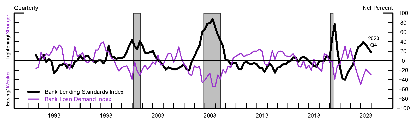
Note: The Bank Lending Standards Index (the black line) and the Bank Loan Demand Index (the purple line) show the net share of banks reporting tighter standards or stronger demand, respectively, aggregated across loan categories by the size of the banks' portfolios in the Call Reports. Positive (negative) values of the two indexes denote either reported net tightening (easing) of lending standards, which is captured by the black line, or reported net strengthening (weakening) of loan demand, which is captured by the purple line. Gray shaded bars denote periods of recession as dated by the National Bureau of Economic Research: 2001:Q2–2001:Q4, 2008:Q1–2009:Q2, and 2020:Q1–2020:Q2.
Source: Federal Reserve Board, Senior Loan Officer Opinion Survey on Bank Lending Practices; Federal Financial Institutions Examination Council, Consolidated Report of Conditions and Income (Call Report); Authors' calculations.
These indices provide a view of how lending conditions and loan demand evolve along the business cycle and have been shown to be predictive of macroeconomic conditions (Bassett et al., 2014). One inherent feature of reported changes in bank lending standards is that they may be influenced by macroeconomic, financial, or economy-wide factors that simultaneously affect the supply of and demand for loans. Thus, attempting to estimate the effects of changes in bank credit supply on the economy using the aggregate index of bank lending standards entails a key identification challenge. In this note, we describe an approach that addresses this challenge and allows us to isolate changes in lending standards driven by independent shifts in the supply conditions of bank credit from those influenced by changes in macroeconomic and financial conditions, bank-level variables, and reported variations in borrower loan demand. Such measure of "shocks" to credit supply can then be used to estimate the independent effects of bank credit supply on real activity. We refer to this measure of shocks to bank credit supply as credit supply indicator (CSI).
Bank-Level Credit Standards Regressions
Our goal is to show how to construct a time series that captures shocks to banks' credit supply. Such series should satisfy some necessary characteristics. It should be uncorrelated with past changes in bank lending standards and bank-level variables that could have persistent or delayed effects on the supply for credit. The series should also be orthogonal to changes in macroeconomic conditions or demand-side factors that could be contemporaneously affecting changes in bank lending standards reported in the survey.5
Toward this goal, we follow Bassett et al. (2014) and regress the index of changes in standards for core loans on its own lag, contemporaneous changes in loan demand, a set of macroeconomic and financial variables aimed at capturing changes in contemporaneous and expected economic conditions, and a set of lagged bank-level variables.6 Relative to Bassett et al. (2014), we extend their analysis by considering a different set of bank-specific variables that could affect banks' reported changes in standards with a lag.7 We also consider a longer sample period to assess the changes in the supply of bank credit implied by banking sector developments in the most recent years.
The variables related to contemporaneous macroeconomic conditions include contemporaneous changes in real GDP, the unemployment rate, the excess bond premium, the real federal funds rate, and measures of macroeconomic and financial uncertainty.8 The variables related to expected macroeconomic conditions are from the Survey of Professional Forecasters and include expectations over the subsequent four quarters about changes in real GDP and unemployment, as well as changes in the 3-month Treasury bill yield and in the 10-year Treasury bond yield. Bank-level variables are all lagged by one quarter and include changes in net interest margins and loan loss provisions, as well as the share of core loans over total assets, the share of core deposits to total assets, the return on assets, the relative size of the bank measured in terms of total assets at a given quarter, and its Tier 1 capital ratio.9 The regressions also include bank fixed effects to capture bank-specific unobservable characteristics that could systematically affect how banks report changes in standards.10 The sample period ranges from 1991:Q2 to 2023:Q4.
In Table 1, we show the results, with each column summarizing a different regression specification. The specification displayed in the first column includes only lagged changes in standards, contemporaneous changes in demand, and the bank fixed effects. The point estimates are statistically significant and economically meaningful, with changes in standards showing some degree of persistence. Furthermore, these variables together already show a sizeable explanatory power, as displayed by a within R2 of 33 percent.11
Table 1: Changes in Bank Lending Standards Regressions
| (1) | (2) | (3) | (4) | |
|---|---|---|---|---|
| Lagged change in standards: ΔSi,t−1 | 0.504*** | 0.404*** | 0.393*** | 0.378*** |
| (34.14) | (26.81) | (25.42) | (24.75) | |
| Change in DI of loan demand: ΔDi,t | -0.127*** | -0.100*** | -0.0964*** | -0.0984*** |
| (-11.79) | (-9.89) | (-9.73) | (-9.69) | |
| Economic Outlook: Et−1[yt+4−yt] | -1.793* | -2.380** | -3.659*** | |
| (-1.95) | (-2.22) | (-3.42) | ||
| Economic Outlook: Et−1[ut+4−ut] | 2.195* | 1.433 | 0.299 | |
| (1.96) | (1.11) | (0.24) | ||
| Economic Outlook: Et−1[r3mt+4−r3mt] | 0.657 | 0.241 | 1.144 | |
| (0.62) | (0.24) | (1.14) | ||
| Economic Outlook: Et−1[r10yt+4−r10yt] | -14.27*** | -13.78*** | -14.45*** | |
| (-7.12) | (-6.40) | (-6.49) | ||
| Change in real GDP: [yt−yt−4] | -2.893*** | -2.880*** | -3.667*** | |
| (-9.44) | (-9.33) | (-11.02) | ||
| Change in unemployment: [ut−ut−4] | 1.045** | 0.774* | 0.291 | |
| (2.33) | (1.67) | (0.61) | ||
| Change in EBP: ΔEBPt | 6.071*** | 5.978*** | 14.85*** | |
| (5.61) | (5.49) | (12.72) | ||
| Change in real FF rate: Δrfft | -3.755*** | -3.369*** | -5.274*** | |
| (-5.29) | (-4.75) | (-7.16) | ||
| Change in macro uncertainty: ΔMUC3mt | 79.05*** | 81.43*** | ||
| (8.38) | (8.37) | |||
| Change in financial uncertainty: ΔFUC3mt | 8.413 | 9.181 | ||
| (1.01) | (1.10) | |||
| Change in NIMs: ΔNIMSi,t−1 | -1.592* | -1.286 | ||
| (-1.88) | (-1.48) | |||
| Change in LLPs: ΔLLPsi,t−1 | 1.688* | 0.578 | ||
| (1.69) | (0.58) | |||
| Share of core loans: CoreLnsi,t−1 | 0.167 | 0.207* | ||
| (1.65) | (1.93) | |||
| Share of core deposits: CoreDepi,t−1 | -0.0509 | 0.00399 | ||
| (-0.46) | (-0.03) | |||
| Return on assets: ROAi,t−1 | 1.866 | 2.114 | ||
| (1.27) | (1.40) | |||
| Bank relative size: Sizei,t−1 | 2.005 | 1.879 | ||
| (1.51) | (1.32) | |||
| Tier 1 capital ratio: Tier1i,t−1 | -1.334*** | -1.341*** | ||
| (-2.98) | (-2.87) | |||
| Change in VIX: ΔVIXt | -0.318*** | |||
| (-3.32) | ||||
| Intercept | 3.502*** | 4.765*** | 4.832*** | 5.015*** |
| (33.46) | (38.54) | (35.31) | (36.95) | |
| Bank fixed effects | Yes | Yes | Yes | Yes |
| R2 | 0.365 | 0.434 | 0.438 | 0.429 |
| Within R2 | 0.331 | 0.403 | 0.408 | 0.398 |
| Number of Observations | 7204 | 7110 | 7110 | 7110 |
Note: t statistics in parentheses. * p < 0.10, ** p < 0.05, *** p < 0.001. Column (1) shows results from a regression including only past changes in standards and contemporaneous changes in demand. Column (2) adds macroeconomic variables. Column (3) further includes lagged bank-level variables. Column (4) is the same specification as in column (2), except that uncertainty measures are substituted with quarterly changes in the VIX index. The dependent variable in all regressions is a bank's change in lending standards across the four core loan categories, weighted by the share of each loan category on the bank's balance sheet. The sample period is from June 1991 until December 2023, and it excludes banks with less than 20 quarters of data.
Source: Federal Reserve Board, Senior Loan Officer Opinion Survey on Bank Lending Practices; Federal Reserve Bank of St. Louis, Federal Reserve Economic Data (FRED), Federal Reserve Bank of Philadelphia, Survey of Professional Forecasters, Federal Financial Institutions Examination Council, Consolidated Report of Conditions and Income (Call Report); Authors' calculations.
Adding the set of macroeconomic variables to the set of regressors allows to improve the explanatory power of the regression, with the within R2 increasing by about seven percentage points, as displayed in the second column of Table 1. The point estimates for the coefficients associated with lagged standards and contemporaneous changes in demand are somewhat lower in size but remain statistically significant. Furthermore, the signs of the estimated coefficients associated with the additional macroeconomic variables are generally consistent with economic intuition: stronger realized and expected economic activity is associated with easier standards, while a larger excess bond premium as well as a higher degree of economic and financial uncertainty are associated with tighter standards.
The third column of Table 1 also shows the regression results obtained by including the set of bank-level variables. The signs of the estimated coefficients for the additional regression variables are also generally consistent with economic intuition. However, most of the estimated coefficients are not statistically significant, while the within R2 increases only marginally. This should not be surprising given that the regression already controls for lagged changes in SLOOS standards at the bank level. It is worth noting that in all specifications the overall R2 is only 3 percentage points higher than the within R2, suggesting a limited explanatory power stemming from bank fixed effects.12 It is also worth pointing that, although bank-level variables and bank fixed effects have a somewhat limited explanatory power (in terms of their contribution to the overall R2), a significant portion of changes in SLOOS standards can be explained by a bank's own lagged standards.
In the fourth column of Table 1, we show the results obtained by substituting the uncertainty measure variables with quarterly changes in the VIX expected equity market volatility index.13 As shown in the table, the R2 remains about unchanged.
As robustness exercises, we considered a range of alternative regression specifications by (i) including quarterly contemporaneous changes in the VIX index jointly with the measures of economic and financial uncertainty, (ii) considering all variables from our baseline regression in lagged terms, (iii) excluding bank-level variables (while keeping lagged SLOOS standards and contemporaneous demand changes). In all these cases, the values and the statistical significance of the point estimates are generally little changed, and, consequently, also our construction of the credit supply shock series.
In the analysis that follows, we consider the specification from the fourth column of Table 1 to be our baseline, since it is the one that allows for more frequent updates. Based on projections from this baseline regression, in Figure 2 we provide a decomposition of what drives changes in lending standards as reported in the SLOOS. The black solid line denotes the aggregate SLOOS series of reported changes in standards, while each of the bars in the figure captures the portion of SLOOS explained by the set of bank-level variables (the light green bars), the set of macroeconomic and financial variables (the orange hatched bars), contemporaneous changes in demand (the purple bars), and lagged standards (the light blue bars). The sum across each of these bars represents the overall value of the SLOOS index predicted by the baseline regression, as depicted by the black dashed-and-dotted line. The main takeaway of this decomposition is that, taken together, past changes in standards and the set of macroeconomic and financial variables play a key role in explaining the dynamics of changes in SLOOS standards. This result is consistent with the results shown in Table 1, in which lagged standards and macroeconomic and financial variables exhibit the largest economic and statistical significance among all explanatory variables, as well as the biggest incidence on the within R2.
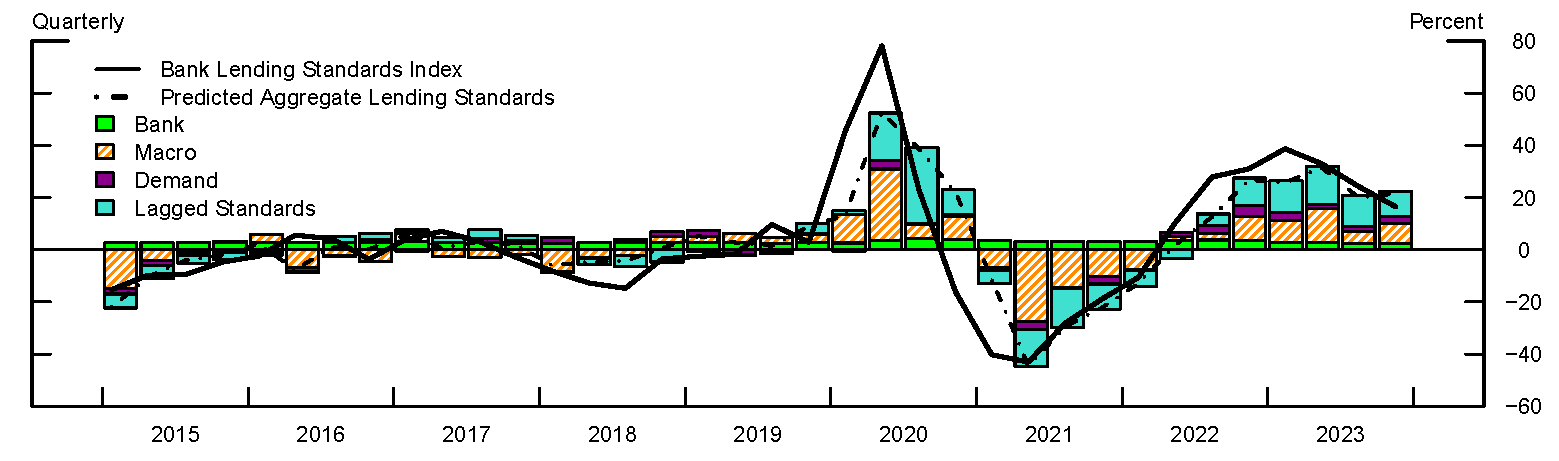
Note: The Bank Lending Standards Index (the black solid line) shows the net share of banks reporting tighter standards aggregated across loan categories weighted by the size of banks' portfolios in the Call Report. The Predicted Aggregate Lending Standards Index (the black dashed-and-dotted line) shows the weighted net share of banks reporting tighter lending standards predicted by a model that incorporates macroeconomic, financial, demand-side, and bank-specific factors using the estimated coefficients from the regression specification shown in the fourth column of Table 1. "Bank" (the light green bars) refers to the predicted component explained by bank fixed effects, banks' changes in net interest margins, changes in loan loss provisions, the share of core loans, the share of core deposits, the return on assets, relative size, and Tier 1 capital ratio; "Macro" (the orange hatched bars) refers to the predicted component explained by contemporaneous changes in real GDP, unemployment rate, excess bond premium, real federal funds rate, and VIX index, as well as four-quarter ahead expected changes in real GDP, unemployment rate, 3-month Treasury bill yield, and 10-year Treasury bond yield. "Demand" (the purple bars) refers to the predicted component explained by contemporaneous changes in demand; and "Lagged Standards" (the light blue bars) refers to the predicted component explained by past changes in lending standards.
Source: Federal Reserve Board, Senior Loan Officer Opinion Survey on Bank Lending Practices; Federal Reserve Bank of St. Louis, Federal Reserve Economic Data (FRED), Federal Reserve Bank of Philadelphia, Survey of Professional Forecasters, Federal Financial Institutions Examination Council, Consolidated Report of Conditions and Income (Call Report); Authors' calculations.
Credit Supply Indicators
Having studied the main drivers of changes in SLOOS standards, we next construct our bank credit supply indicators. To this end, we adjust reported changes in banks' lending standards to account for the influence of the set of factors described above by computing the residuals from the bank-level regression specified in the fourth column of Table 1. We then aggregate the estimated residuals across banks using as weights the share of a bank's core loan portfolio over the total of core loans on banks' balance sheets. Figure 3 shows the results, with the black line denoting the net share of banks reporting tighter standards (i.e., the original SLOOS series) and the red line depicting our aggregate credit supply indicator. Both the SLOOS index for changes in standards and the CSI series tend to increase before the onset of recessions, amid concerns about economic uncertainty and reduced risk tolerance.14 However, given the adjustment procedure described above, the CSI displays a much lower degree of persistence.
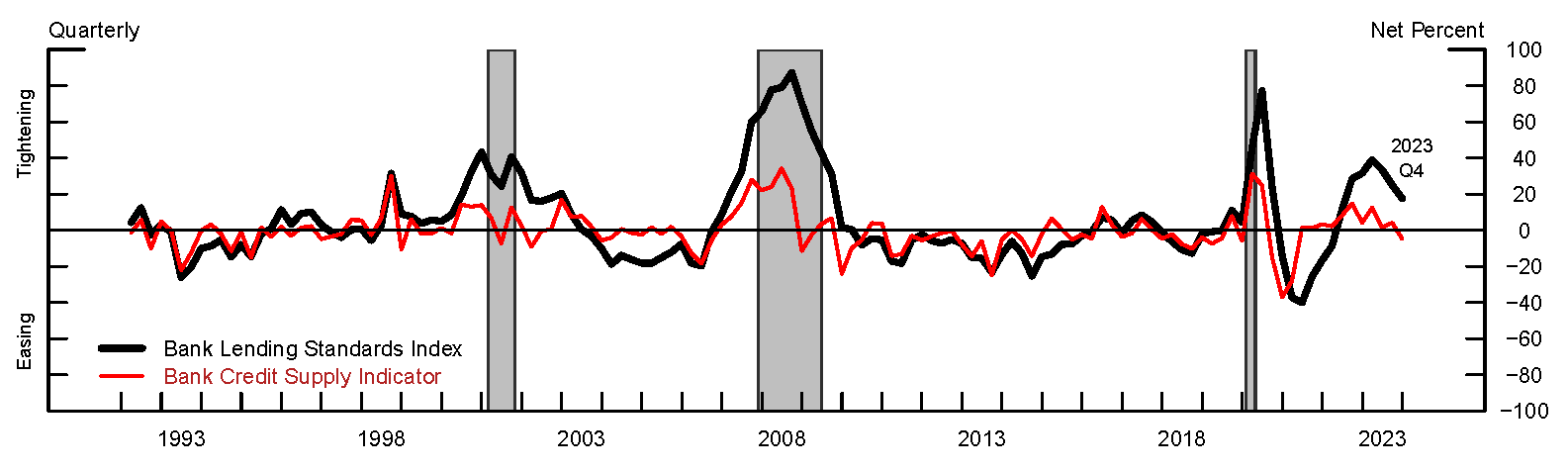
Note: The Bank Lending Standards Index (the black line) shows the net share of banks reporting tighter standards aggregated across loan categories weighted by the size of banks' portfolios in the Call Report. The Bank Credit Supply Indicator (the red line) shows the weighted net share of banks reporting tighter standards, after adjusting for macroeconomic, financial, demand-side, and bank-specific factors using the estimated coefficients from the regression specification shown in the fourth column of Table 1. Gray shaded bars denote periods of recession as dated by the National Bureau of Economic Research: 2001:Q2–2001:Q4, 2008:Q1–2009:Q2, and 2020:Q1–2020:Q2.
Source: Federal Reserve Board, Senior Loan Officer Opinion Survey on Bank Lending Practices; Federal Reserve Bank of St. Louis, Federal Reserve Economic Data (FRED), Federal Reserve Bank of Philadelphia, Survey of Professional Forecasters, Federal Financial Institutions Examination Council, Consolidated Report of Conditions and Income (Call Report); Authors' calculations.
One episode of particular importance for the U.S. economy in 2023 was the collapse of Silicon Valley Bank (SVB) and the subsequent stress in the banking sector during the first quarter of the year. In fact, Figure 3 shows a widespread tightening in standards reported in the April 2023 SLOOS survey. The implied value for the CSI points to a moderately-sized shock stemming from the banking developments occurred between the January and April 2023 SLOOS surveys, equivalent to an 11 percentage-point increase in the net percentage of banks reporting tighter lending standards, or one-half standard deviation of the SLOOS historical series for changes in bank lending standard. In the subsequent July and October surveys, the CSI shows that the continued net tightening in bank lending standards was generally in line with what might be expected given the historical relationship between bank lending standards and macroeconomic conditions.15
One appealing feature of the methodology described above is that it can also be used to compute time series for the CSI across the various bank loan categories, namely, commercial and industrial (C&I), commercial real estate (CRE), residential real estate (RRE), and consumer loans. For each loan category, we adjust the regression variables accordingly. In particular, we use changes in standards for the loan category of reference as the dependent variable. Regarding the explanatory variables, the lagged changes in standards, the contemporaneous changes in demand, and the share of loans over total assets are adjusted to represent the loan category of reference, while all other explanatory variables are unchanged.
In Figure 4, we show the results for each loan category. Panels (a) through (d) display results for C&I, CRE, RRE, and consumer loans, respectively. As in Figure 3, the black line represents changes in standards as measured from SLOOS, while the red line denotes the CSI measure for the respective loan category. The figure reveals a few common patterns around the last two recessions for the SLOOS series of changes in standards and the CSI measures, with these series increasing ahead of these recessions.16 However, there are also meaningful differences across the various loan categories. For instance, the CSI index for RRE loans was much more persistent during the Great Financial Crisis (GFC) than for the other categories. In contrast, the net percentage of banks reporting tighter standards was lower for RRE loans than for other categories during the SVB episode. Arguably, this difference reflects that fact that standards for RRE were already at elevated levels, following several quarters of reported net tightening after the GFC. It is also worth noting that, in contrast to changes in standards, the CSI series are weakly correlated across loan categories.17
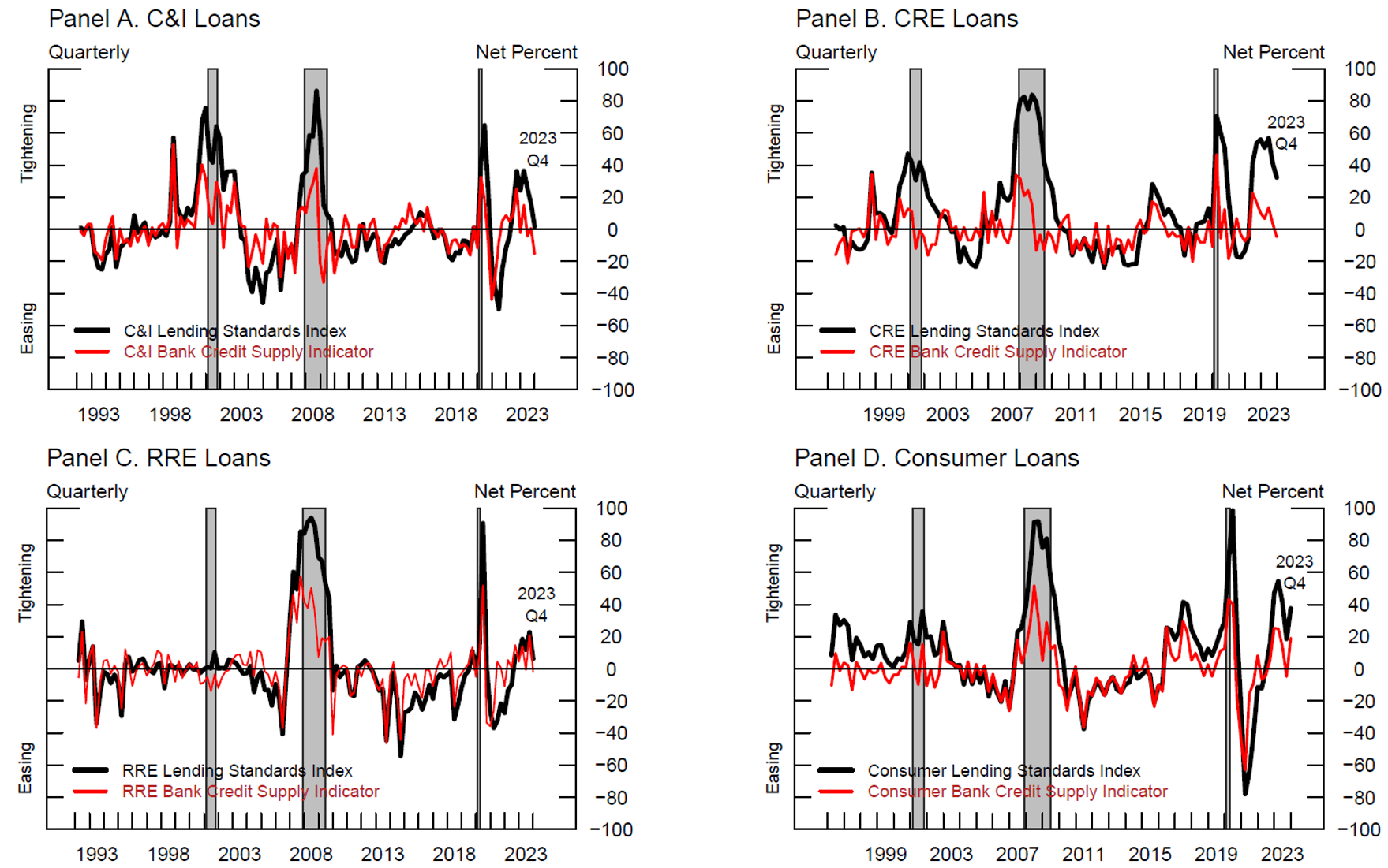
Note: The C&I, CRE, RRE, and Consumer Lending Standards Indexes (the black solid lines in Panels A through D) show the net share of banks reporting tighter standards aggregated across the respective loan categories weighted by the size of banks' corresponding loan portfolios in the Call Report. The C&I, CRE, RRE, and Consumer Bank Credit Supply Indicators (the red solid lines in Panels A through D) show the weighted net share of banks reporting tighter standards for loan in the respective categories, after adjusting for macroeconomic, financial, demand-side, and bank-specific factors using the estimated coefficients from the regression specification shown in the fourth column of Table 1. Gray shaded bars denote periods of recession as dated by the National Bureau of Economic Research: 2001:Q2–2001:Q4, 2008:Q1–2009:Q2, and 2020:Q1–2020:Q2.
Source: Federal Reserve Board, Senior Loan Officer Opinion Survey on Bank Lending Practices; Federal Reserve Bank of St. Louis, Federal Reserve Economic Data (FRED), Federal Reserve Bank of Philadelphia, Survey of Professional Forecasters, Federal Financial Institutions Examination Council, Consolidated Report of Conditions and Income (Call Report); Authors' calculations.
As a final robustness check, in Figure 5 we observe how the baseline CSI series for core loans (the red line) compares with an aggregated CSI series across loan categories (the black dashed-and-dotted line), with the CSI from each category weighted according to the share of each corresponding loan type over core loans on banks' balance sheets. For a large part of the sample period, the two series are remarkably similar in both levels and dynamics. This observation is useful should a researcher be interested in doing an in-depth cross-category analysis with aggregate implications.
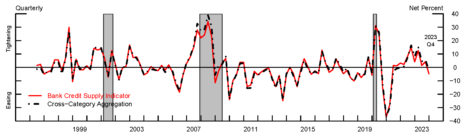
Note: The Bank Credit Supply Indicator (the red solid line) shows the weighted net share of banks reporting tighter standards, after adjusting for macroeconomic, financial, demand-side, and bank-specific factors using the estimated coefficients from the regression specification shown in the fourth column of Table 1. The Cross-Category Aggregation CSI (the black dashed-and-dotted line) shows the aggregation across lending categories of category-weighted net share of banks reporting tighter standards, after adjusting for macroeconomic, financial, demand-side, and bank-specific factors using the estimated coefficients from the regression specification shown in the fourth column of Table 1. Gray shaded bars denote periods of recession as dated by the National Bureau of Economic Research: 2001:Q2–2001:Q4, 2008:Q1–2009:Q2, and 2020:Q1–2020:Q2.
Source: Federal Reserve Board, Senior Loan Officer Opinion Survey on Bank Lending Practices; Federal Financial Institutions Examination Council, Consolidated Report of Conditions and Income (Call Report); Authors' calculations.
Conclusion
In this note, we described a method for gauging shocks to bank's credit supply, or credit supply indicators, across a range of loan categories, using the Federal Reserve's Senior Loan Officer Opinion Survey. These measures can provide a useful tool to assess whether the survey responses from banks point to excess tightening or easing relative to the historical empirical relationship between banks' lending standards, borrowers' demand for loans, bank characteristics, and the macroeconomic and financial environment. In a companion note (Cavallo, Morelli, and Zarutskie, 2024), we use these credit supply indicators to examine the possible macroeconomic implications of bank credit supply shocks.
References
Bernanke, Ben S., Mark Gertler, and Simon Gilchrist (1996). "The Financial Accelerator and the Flight to Quality," Review of Economic and Statistics, vol. 78 (February), pp. 1–15.
Bernanke, Ben S. (2018). "The Real Effects of Disrupted Credit: Evidence from the Global Financial Crisis," Brookings Papers on Economic Activity, Fall, pp. 251–322.
Bassett, William F., Mary Beth Chosak, John C. Driscoll, and Egon Zakrajšek (2014). "Changes in Bank Lending Standards and the Macroeconomy," Journal of Monetary Economics, vol. 62 (March), pp. 23–40.
Carlson, Mark A., Thomas King, and Kurt F. Lewis (2011). "Distress in the Financial Sector and Economic Activity," B.E. Journal of Economic Analysis and Policy, vol. 11: Iss. 1 (Contributions), Article 35.
Cavallo, Michele, Juan M. Morelli, and Rebecca Zarutskie (2024). "Unpacking the Effects of Bank Credit Supply Shocks on Economic Activity," FEDS Notes. Washington: Board of Governors of the Federal Reserve System, May 24.
Favara, Giovanni, Simon Gilchrist, Kurt F. Lewis, Egon Zakrajšek (2016). "Updating the Recession Risk and the Excess Bond Premium," FEDS Notes. Washington: Board of Governors of the Federal Reserve System, October 6.
Glancy, David, Robert Kurtzman, and Rebecca Zarutskie (2020). "An Aggregate View of Bank Lending Standards and Demand," FEDS Notes. Washington: Board of Governors of the Federal Reserve System, May 4.
Jurado, Kyle, Sydney C. Ludvigson, and Serena Ng (2015). "Measuring Uncertainty," American Economic Review, vol. 105 (March), pp. 1177–1216.
1. We thank Stephanie Aaronson and Rochelle Edge for thoughtful comments. The analysis and conclusions set forth are those of the authors and do not indicate concurrence by the Board of Governors of the Federal Reserve System. Any errors or omissions are the responsibility of the authors. Return to text
2. References on this topic include, among many others, Bernanke, Gertler, and Gilchrist (1996), Carlson, King, and Lewis (2011), Bassett, Chosak, Driscoll, and Zakrajšek (2014), and Bernanke (2018). Return to text
3. See https://www.federalreserve.gov/data/sloos.htm. The survey has been asked consistently since 1990 but was started in the 1960s. Return to text
4. For a detailed description of the aggregate index of bank lending standards, see Glancy, Kurtzman, and Zarutskie (2020). Return to text
5. The consideration of demand-side factors addresses concerns about identification issues by which both demand- and supply-side factors could be potentially affecting banks' reported changes in standards. Return to text
6. The inclusion of expectations about macroeconomic conditions also helps mitigate the identification concern by which banks may adjust standards in response to changes in the macroeconomic outlook. See Bassett et al. (2014) for a brief discussion on this topic. Return to text
7. In particular, we include bank-level capitalization, a variable that might also affect bank lending standards, and we substitute changes in stock prices with changes in the return on assets (ROA), which allows us to keep in our sample the smaller banks that are not publicly listed. Return to text
8. The excess bond premium is obtained from Favara, Gilchrist, Lewis, and Zakrajšek (2016). The indicators for macroeconomic and financial uncertainty indicators are obtained from Jurado, Ludvigson, and Ng (2015). Return to text
9. Core deposits are defined to be small time deposits (i.e., deposits of less than $100,000). Return to text
10. Bassett et al. (2014) cite as examples biases towards tightening or the effects of banking relationships. Return to text
11. The within R2 measures how much of the variance within the panel units the model does account for. It thus captures the explanatory power of the model after controlling for bank fixed effects. Return to text
12. The higher overall R2 is consistent with a meaningful degree of heterogeneity in estimated bank fixed effects (not shown). Return to text
13. One motivation for substituting the uncertainty measure variables with changes in the VIX index is that the latter is available at a higher frequency, and it also allows for more timely re-estimation of the econometric model. Return to text
14. Gray shaded bars denote periods of recession as dated by the National Bureau of Economic Research. i.e., 2001:Q2–2001:Q4, 2008:Q1–2009:Q2, and 2020:Q1–2020:Q2. Return to text
15. It is important to note that, while the CSI series basically shows no additional credit supply shock in the July 2023 survey, the SLOOS series of changes in standards exhibits a significant degree of persistence, implying that the shock measured in the aftermath of the SVB collapse likely continued to have an impact on reported changes in lending standards in the subsequent quarters. Return to text
16. The 2001:Q2–2001:Q4 recession was different, in that the net percentages of banks reporting tighter lending standards were much larger for business (C&I and CRE) loans than for household (RRE and consumer) loans. Return to text
17. The correlation ranges from 12 percent (between the C&I and RRE measures) to 50 percent (between C&I and CRE). In turn, the correlation for changes in standards ranges from 50 percent (between C&I and RRE) to 76 percent (between C&I and CRE). Of note, standard deviations for changes in standards are similar, around 25 percent, while for the CSI measures standards deviations range from 11 percent to 16 percent. Return to text
Cavallo, Michele, Juan Morelli, Rebecca Zarutskie, and Solveig Baylor (2024). "Measuring Bank Credit Supply Shocks Using the Senior Loan Officer Survey," FEDS Notes. Washington: Board of Governors of the Federal Reserve System, May 24, 2024, https://doi.org/10.17016/2380-7172.3516.
Disclaimer: FEDS Notes are articles in which Board staff offer their own views and present analysis on a range of topics in economics and finance. These articles are shorter and less technically oriented than FEDS Working Papers and IFDP papers.