FEDS Notes
March 25, 2025
Underlying Inflation: An Ensemble Averaging Approach
Gianni Amisano, Travis Berge, and Simon C. Smith*
1. Introduction
Underlying inflation (ULI) is the rate of inflation we expect to prevail in the absence of resource slack, supply shocks, and other temporary disturbances to inflation. ULI is therefore critical to determining the contour of inflation. However, ULI is an unobserved variable that has proven elusive to pin down. Generating accurate estimates of ULI is therefore of paramount importance, but very challenging.
Estimates of ULI are highly uncertain, especially estimates of ULI in recent history, which are the most informative for policy-makers. Given a particular model, one can derive and report point estimates for ULI as well as confidence intervals that capture uncertainty surrounding that model-specific estimate. However, this measure of uncertainty overstates how confident we should be about a given ULI estimate, because we do not know which individual model is the "true" model, if indeed such a thing exists. When this "model uncertainty" is high, it is sensible to consult a range of models. The intuition for such an approach is that while some models will systematically overestimate ULI, others will underestimate it. The model-specific errors even out as we average these estimates.1
In this note we estimate ULI from a suite of models and take an average of their estimates to provide an ensemble ULI estimate that will likely provide more robust estimates than even the best individual model. This ensemble ULI estimate is a useful benchmark to monitor movements in actual inflation, and helps inform the contour of expected future inflation.
We consider seven estimates of ULI that are obtained from different models and information sets. The most relevant information is realized inflation and inflation expectations, but our model set includes models that condition on macroeconomic conditions more broadly. Specifically, our model suite includes two moving averages of realized inflation, three models that use information on both realized inflation and inflation expectations, a time-varying parameter Vector Autoregressive model (TVP-VAR) that models jointly the dynamics of inflation, relative price inflation of imports and energy, and the unemployment gap, and a small macroeconometric model that estimates ULI in conjunction with the trends in output and the unemployment rate.
With the individual ULI estimates in hand, we must next determine how to combine them. One possibility would be to evaluate each model's inflation forecast accuracy and weight the models proportionally to their forecast ability. However, the optimal weights are likely to vary through time. Although numerous methods have been proposed to estimate time-varying weights (e.g., Bayesian model averaging or dynamic model averaging), the available sample size for such an exercise is likely too small to discriminate amongst the various models since estimating the weights induces another layer of estimation error into what is already a highly uncertain environment. Indeed, in many empirical applications, these weights are so unstable that the advantage of model averaging is more than offset by the additional error from estimation of the weights (Clemen (1989), Stock and Watson (2004), Amisano and Geweke (2017)). For these reasons, we propose an ensemble ULI estimate that is simply the equal-weighted average of the seven individual ULI estimates.
2. Suite of Individual ULI Estimates
Table 1 summarizes the models we use in our ULI ensemble. The models we use are not comprehensive but do encompass a number of sensible approaches and data for estimating underlying inflation. We provide details of the models, data, and estimation in the technical appendix.
The first approach to estimating ULI is also the simplest. In this approach, ULI is backwards looking, and is estimated as the sample mean of quarterly core PCE price inflation over either 15 years or 25 years.
The second approach jointly models actual inflation and a measure of expected future inflation. Thus, ULI is no longer purely backwards-looking; instead, it is the driver of common movements in realized and a measure of expected future inflation. Specifically, we apply the time-varying parameter unobserved components stochastic volatility (TVP-UCSV) model of Chan et al. (2018), a more general version of the well-known UCSV model from Stock and Watson (2007). It allows the wedge between the measure of expected inflation and ULI to vary over time, allowing for incomplete pass-through of expectations into ULI. We estimate three versions of this model, each of which uses a different measure of long- run inflation expectations. Specifically, we consider long-run expectations from Michigan, the Index of Common Inflation Expectations projected onto Michigan expectations (Ahn and Fulton 2020), and inflation compensation derived from Treasury Inflation-Protected Securities (TIPS).2
Table 1: ULI ensemble model suite
| Model type | Key data | Estimation strategy |
|---|---|---|
| Univariate averages | ||
| 15-year rolling mean | Realized inflation | Simple mean |
| 25-year rolling mean | Realized inflation | Simple mean |
| Joint models of realized and expected inflation | ||
| Chan et al. (2018) | Realized and Michigan expected inflation TVP-UCSV Chan et al. (2018) | Realized and CIE expected inflation |
| Macroeconomic models | ||
| Clark and Terry (2010) | Realized inflation, un. rate gap | TVP-VAR UC-3 |
Notes: Table summarizes the seven models included in the ULI ensemble suite. Models are estimated at the quarterly frequency, and unless otherwise noted, realized inflation is measured by the annualized change in the core PCE price index. UC denotes unobserved component model; TVP-UCSV is time-varying parameter unobserved component with stochastic volatility.
The third class of models are multivariate models that jointly model nominal and real economic outcomes. The first of these is a flexible and general reduced-form model, based on Clark and Terry (2010). Specifically we estimate a time-varying parameter vector autoregressive (TVP-VAR) model on core PCE price inflation, relative import price inflation, relative energy price inflation, and the unemployment gap from the Congressional Budget Office. The model is intended to be completely reduced-form; while the time-varying coefficients allow for slow-moving changes to the covariances and variances of the shocks to the VAR. The final ULI estimate comes from a stylized semi-structural unobserved component model estimated on real GDP, the unemployment rate, and core PCE price inflation, denoted UC-3. The model explicitly embeds important macroeconomic relationships, such as an Okun's law and Phillips curve (see, e.g., Clark (1987), Sinclair (2009), and Barbarino et al. (2024)). The difference between realized inflation and ULI is proportional to the model's output gap estimate. ULI is modeled as a weighted sum of long-run inflation expectations (the 5-to-10 year forward expectation for PCE prices from the SPF) and an unobserved trend.
3. Results
Figure 1 graphs the evolution of our ensemble ULI estimate between 2005:Q1 and 2024:Q4 and the four-quarter percent change in the core PCE price index. ULI steadily declines from 2.2 percent in 2005 through 2015. At that point, ULI hovers at a trough of roughly 1.8 percent until inflation picks up following the pandemic. The figure plots ULI estimates as the models estimate them having seen the data through 2024:Q4; i.e., they are not real-time estimates. However, the real time estimates are very similar to the full sample estimates, reflecting a key advantage of our ensemble ULI estimate: unlike some popular individual models (such as the UCSV model (Stock and Watson 2007) or the TVP-AR model (Cogley and Sargent 2005)), because the ensemble is an average of many different individual estimates, it typically does not show large historical revisions. This makes it more informative for policymakers making decisions in real time. The uncertainty around the ULI estimate is measured by an approximate 70 percent confidence interval (the red shaded region in the figure), which is computed as the equally weighted average of the 70 percent confidence interval of each individual ULI estimate. Prior to the pandemic-related recession, the uncertainty surrounding the estimate is relatively moderate, with the interval spanning a range from 1.6-2.0 percent in the 2015–2019 period.
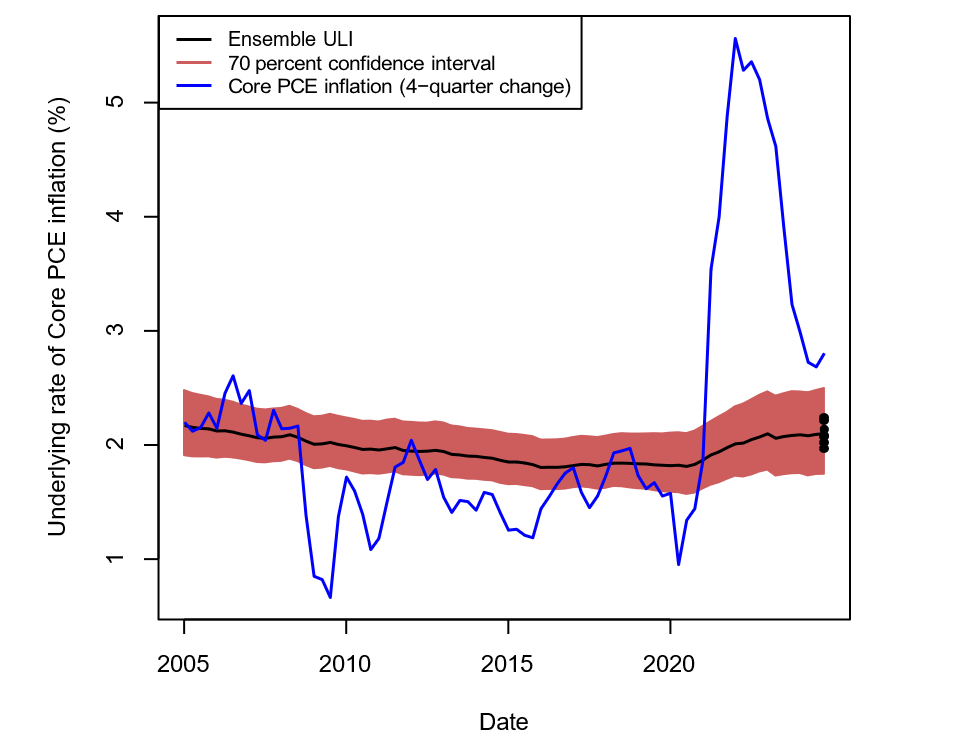
Notes: The black line in this figure graphs the evolution of the ensemble (equal-weighted) average of the seven different individual ULI estimates. The red colored polygon denotes the 70 percent confidence interval around this estimate. The blue line is the four-quarter percent change in the core PCE price index. See text for details.
Figure 2 zooms in on the estimates since 2019:Q1. ULI moved higher alongside inflation in the post-pandemic period, reaching 2.1 percent in 2022:Q3, roughly its level in 2006-2008. It subsequently moved sideways, remaining at 2.1 percent through 2024:Q4. Even in light of its increase, the estimate of ULI remains close to the Federal Reserve's two percent inflation target. Indeed, the individual ULI estimates that comprise the ensemble (black circles) are clustered between 2.0 and 2.2 percent in the final quarter. These estimates suggest that once all transitory inflationary shocks dissipate, inflation should settle around two percent.
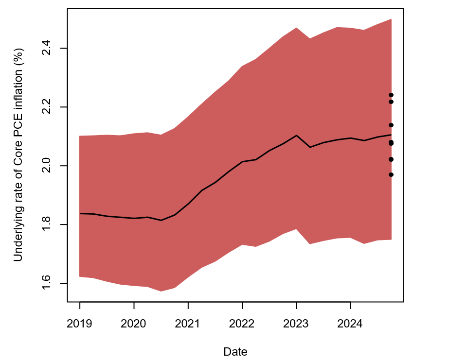
Notes: The black line is the equally-weighted average of the individual ULI estimates. The red shaded area denotes an approximated 70 percent confidence interval around this estimate. The black circles denote the individual ULI estimates in the final quarter of the sample, 2024:Q4. See text for details.
The 70 percent credible intervals shown in Figure 2 capture the magnitude of risks around ULI. The ensemble suggests an increase in the uncertainty around ULI between 2021 and 2024, as the width of the credible set increased from 0.5 to 0.75 percentage point. In addition, by construction, the uncertainty bands around the ULI estimate are symmetric, i.e., implicitly they assume the risks around ULI are balanced. To investigate whether the balance of risks around ULI changed during the pandemic, Figure 3 displays a box-and-whisker plot of the individual ULI estimates. The horizontal line within each box denotes the median estimate in a given quarter, and the colored box covers the interquartile range of the estimates. The dashed lines that extend out of the colored boxes denote the minimum and maximum estimates.
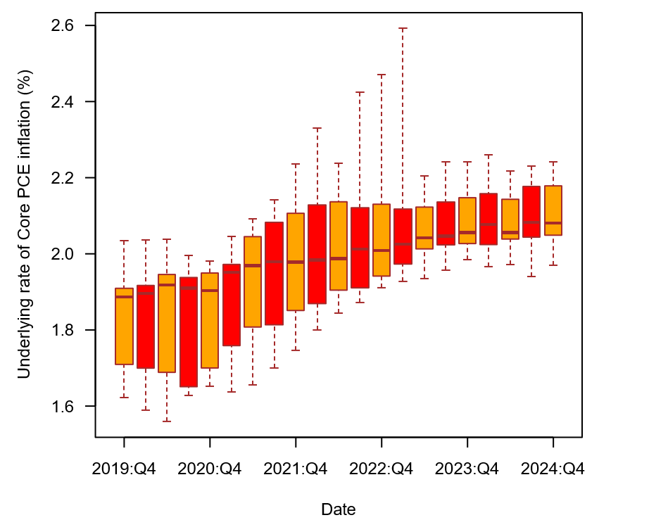
Notes: This figure presents a box-and-whisker plot of the model ULI estimates from 2019:Q1 through 2024:Q4. The colored box covers the interquartile range, the dashed lines that extend out of the colored boxes denote the minimum and maximum of the seven ULI estimates. See text for details.
Once again, we see that the magnitude of risks around ULI increased during the pandemic, reflected by the span of the minimum and maximum values increasing and reaching a peak in late-2021 and especially in 2022 at which point the maximum estimates reached as high as 2.6 percent.3 Not only did the magnitude of risks around ULI grow from 2019 to 2022 but, having been fairly balanced in 2019, they became skewed to the upside by 2022. This upside skew is manifest in a few different ways. First, the median estimate is closer to the lower quartile than the upper quartile, especially in the second half of 2021 and 2022. Also note that the distance between the maximum value and the upper quartile is larger than that between the minimum value and the lower quartile. Finally, it is notable that the minimum estimate moved up by more than the median estimate; that is, whereas the median estimate moved from roughly 1.9 percent in 2021:Q1 to 2.1 percent in 2024:Q4, the minimum ULI estimate moved from 1.6 to 2.0 over the same period. Since the end of 2022, risks around ULI have become smaller in magnitude and better balanced. The interquartile range currently covers a narrow range from 2.0 to 2.15 percent with the maximum and minimum values being not far from this range.
In short, our ensemble ULI approach suggests that ULI moved up from 1.8 percent on the eve of the pandemic, peaking at 2.1 percent in 2022. The magnitude of risks around ULI became large over this period and more skewed to the upside. While the estimate of ULI has remained at 2.1 percent since 2022, the risks around it have decreased in magnitude and become better balanced.
More generally, our ensemble ULI approach should be a useful tool for thinking about ULI going forward, particularly if we are entering a more turbulent world with more changes in fundamental economic relations – as speculated by Lagarde (2023).
References
Ahn, H. J. and C. Fulton, "Index of common inflation expectations," FEDS Notes (2020).
Amisano, G. and J. Geweke, "Prediction using several macroeconomic models," Review of Economics and Statistics 99 (2017), 912–925.
Barbarino, A., T. J. Berge and A. Stella, "The stability and economic relevance of output gap estimates," Journal of Applied Econometrics (2024).
Bates, J. M. and C. W. Granger, "The combination of forecasts," Journal of the Operational Research Society 20 (1969), 451–468.
Chan, J. C., T. E. Clark and G. Koop, "A new model of inflation, trend inflation, and long-run inflation expectations," Journal of Money, Credit and Banking 50 (2018), 5–53.
Clark, P. K., "The cyclical component of US economic activity," The Quarterly Journal of Economics 102 (1987), 797–814.
Clark, T. E. and S. J. Terry, "Time variation in the inflation passthrough of energy prices," Journal of Money, credit and Banking 42 (2010), 1419–1433.
Clemen, R. T., "Combining forecasts: A review and annotated bibliography," International Journal of Forecasting 5 (1989), 559–583.
Cogley, T. and T. J. Sargent, "Drifts and volatilities: monetary policies and outcomes in the post WWII US," Review of Economic Dynamics 8 (2005), 262–302.
Kim, D., C. Walsh and M. Wei, "Tips from TIPS: Update and discussions," FEDS Notes (2019).
Lagarde, C., "Policymaking in an age of shifts and breaks," in Proceedings-Economic Policy Symposium-Jackson Hole (Federal Reserve Bank of Kansas City, 2023).
Peneva, E. V. and J. B. Rudd, "The passthrough of labor costs to inflation," Journal of Money, Credit and Banking 49 (2017), 1669–1839.
Sinclair, T. M., "The Relationships between Permanent and Transitory Movements in U.S. Output and the Unemployment Rate," Journal of Money, Credit and Banking 41 (2009).
Stock, J. H. and M. W. Watson, "Combination forecasts of output growth in a seven- country data set," Journal of Forecasting 23 (2004), 405–430.
———, "Why has US inflation become harder to forecast?," Journal of Money, Credit and banking 39 (2007), 3–33.
Appendix A. Model and data details
This appendix provides additional details regarding the suite of models considered.
Table A1 describes sources of the data used and their transformations.
Table A1: Data sources and transformations
| Transformation | Source | |
|---|---|---|
| Core PCE inflation | Annualized percent change | FRED (PCEPILFE) |
| Michigan long-run expected inflation | Annualized percent change | University of Michigan, Survey Research Center, Surveys of Consumers |
| CIE long-run expected inflation | Annualized percent change | Ahn and Fulton, 2020 |
| TIPS inflation compensation | Annualized percent change | KWW, 2019 |
| SPF inflation expectations | Annualized percent change | FRB-Phil. |
| Relative import price inflation | Ratio of import price inflation to core PCE inflation | FRED (PCEPILFE) |
| Relative energy price inflation | Ratio of import price inflation to core PCE inflation | FRED (DNRGRV1Q225SBEA, PCEPILFE) |
| Unemployment rate | Percent | FRED (UNRATE) |
| Natural rate of unemployment | Percent | FRED (NROU) |
| Gross domestic product | FRED (GDPC1) | |
| Gross domestic income | FRED (A261RL1Q225SBEA) |
Models 1 and 2.
The first two models of ULI are simply a sample mean of annualized quarterly core PCE price inflation, with an average taken over the previous 15 or 25 years.
Models 3-5. Time-varying parameter unobserved components stochastic volatility models of inflation and inflation expectations.
We next consider three distinct time-varying parameter unobserved components models with stochastic volatility (TVP-UCSV; Chan et al. (2018)). A TVP-UCSV model filters a trend of inflation from realized inflation and a measure of inflation expectations. The model generalizes the UCSV model of Stock and Watson (2007), allowing for time-varying parameters so that the wedge between expectations and inflation's trend could vary over time. Letting $$\pi_{t}$$ denote quarter-on-quarter core PCE price inflation, $$\pi_{t}^{e}$$ a measure of expected inflation, and $$\pi_{t}^{*}$$ ULI, the model assumes that deviations of inflation from ULI follow an AR(1) process, and expectations are a linear function of trend inflation:
$$$$ \begin{align*} \pi_{t} - \pi_{t}^{*} &= b_{t} (\pi_{t-1} - \pi_{t-1}^{*}) + \sigma_{\epsilon,t}\epsilon_{t}\\ \pi_{t}^{*} &= \pi_{t-1}^{*} + \sigma_{e,t}e_{t} \\ b_{t} &= b_{t-1} + \epsilon_{b,t} \\ \Delta \text{log } \sigma^{2}_{e,t} &= \gamma_{e} v_{e,t}\\ \Delta \text{log } \sigma^{2}_{\epsilon,t} &= \gamma_{\epsilon} v_{\epsilon,t}\\ \epsilon_{b,t} &\sim TN(0, \sigma^{2}_{b}) \end{align*}\ (A.1)$$$$
in which all the time-varying parameters evolve over time as independent random walks, $$\epsilon_{t}, e_{t}, \eta_{t}, v_{\epsilon,t}, v_{e,t} \sim N(0,1)$$, $$\sigma_{\epsilon,t}$$ is observation stochastic volatility, $$\sigma^{2}_{e,t}$$ is trend stochastic volatility, and $$TN(.,.)$$ denotes a Gaussian distribution truncated to keep $$0<b_t<1$$. The three versions of this model each uses a different measure of inflation expectations: long-run expected inflation from the Michigan Survey of Consumers, TIPS inflation compensation, and the Index of Common Inflation Expectations (CIE-Michigan)—a measure constructed from a factor model applied to approximately 10 different measures of expected inflation, and which we treat as observed.
Model 6. Time-varying parameter VARs.
The next model is the time-varying parameter unobserved vector autoregressive (TVP-VAR) model of Clark and Terry (2010). The model is a reduced-form VAR model with time-varying parameters and stochastic volatility, where the information set included in the VAR includes measures of inflation and the difference between the unemployment rate and it's long-run trend as estimated by the CBO. Specifically, Let $$y_t$$ be a column vector containing core PCE price inflation, relative import price inflation, relative energy price inflation, and the unemployment gap from the Congressional Budget Office, the dynamics of which are jointly modelled. Formally, the model is:
$$$$ \begin{align*} y_{t} &= \Phi_{0t} + \Phi_{1t} y_{t-1} + \Phi_{2t} y_{t-2} + \Phi_{3t} y_{t-3} + A _{\epsilon,t}^{*} \Sigma_{\epsilon,t}^{0.5} \eta_{\epsilon,t} \\ \boldsymbol{\Phi}_{t} &= \boldsymbol{\Phi}_{t-1} + Q^{0.5}\zeta_{\Phi,t} \\ a_{i,t} &= a_{i,t-1} + \sigma_{a,i} \zeta_{a,i,t} \\ \Delta \text{log } \sigma^{2}_{\epsilon,i,t} &= \gamma_{\epsilon, i} v_{\epsilon, i,t} \end{align*}\ (A.2)$$$$
in which $$\Sigma_{\epsilon,t} = diag(\sigma^{2}_{\epsilon,1,t}, \ldots, \sigma^{2}_{\epsilon,n,t})$$ and $$\sigma^{2}_{\epsilon,n,t}$$ is observation stochastic volatility, $$A_{\epsilon, t}$$ is a lower diagonal matrix that controls correlations in observation stochastic volatility, $$\eta_{\epsilon, t}, \zeta_{\Phi, t}, \zeta_{a, i, t}, v_{\epsilon, i, t} \sim N(0,1)$$, and $$\boldsymbol{\Phi}_{t} = vec(\Phi_{0,t},\ldots, \Phi_{3,t})$$.
Having estimated the model, we exposit the VAR in state-space form as
$$$$ \begin{equation} \boldsymbol{y}_{t} = \boldsymbol{\mu}_{t} + \boldsymbol{\Psi}_{t}\boldsymbol{y}_{t-1} + \boldsymbol{A}^{*}_{\epsilon, t}\boldsymbol{\Sigma}_{\epsilon, t}^{0.5} \eta_{\epsilon, t} \end{equation}\ (A.3)$$$$
and retrieve trend inflation as the first entry of the vector $$\boldsymbol{\tau}_{t} = (\boldsymbol{I} - \boldsymbol{\Psi}_{t})^{-1} \boldsymbol{\mu}_{t}$$.
Model 7. Small-scale semi-structural unobserved component model.
The final model we consider is a small-scale, semi-structural unobserved component model. The model jointly estimates an output gap, unemployment rate gap and inflation gap, i.e., the deviation of actual inflation from its underlying trend.
Specifically the model is written:
$$$$ \begin{align*} GDP_t &= y^*_t + c_t + e_{GDP t} \\ GDI_t &= y^*_t + c_t + e_{GDI t} \\ y^*_t &= y^*_{t-1} + \tau_t + \varepsilon_{y^* t} \\ \tau_t &= \tau_{t-1} + \varepsilon_{\tau t} \\ c_t &= \phi_1 c_{t-1} + \phi_2 c_{t-2} + \varepsilon_{c t} \\ u_t &= u^*_t + \alpha_0 c_t + \alpha_1 c_{t-1} + e_{u t} \\ u_t &= u^*_t + \varepsilon_{u^* t} \\ \pi_t &= \pi^{LUI}_t + \beta_0 c_t + \beta_1 c_{t-1} + \upsilon Z_t + e_{\pi t} \\ \pi^{LUI}_t &= \gamma E \pi^{SPF}_t + (1-\gamma) \pi^*_t \\ \pi^*_t &= \pi^*_{t-1} + \varepsilon_{\pi^*_t} \end{align*}\ (A.4)$$$$
where GDP denotes 100 times the log of real GDP, GDI represents gross domestic income, $$u$$ the unemployment rate, and $$\pi$$ the annualized percent change in the core PCE price index. $$Z$$ represent additional variables that may help to explain cyclical movements in inflation that are unrelated to the output gap: a measure of core import prices (measured as consumption- weighted core import prices divided by core PCE prices) and relative energy price inflation (the difference between quarterly energy price inflation and core PCE inflation). Expected inflation is the median expectation for PCE price inflation over the next 10 years (see Peneva and Rudd (2017)).
Email addresses: [email protected] (Gianni Amisano), [email protected] (Travis Berge), [email protected] (Simon C. Smith))
The authors thank Jeremy Rudd. Any remaining errors are our own. The views expressed in this paper are those of the authors and do not necessarily reflect the views and policies of the Board of Governors or the Federal Reserve System. Return to text
1. Indeed, ensemble averages typically deliver improved predictive accuracy relative to any of the individual models in the ensemble average because the forecast errors of the individual models average out (Bates and Granger 1969). Return to text
2. Specifically, we use the zero-coupon TIPS breakeven inflation rate obtained from the four-factor model of Kim et al. (2019) that uses smoothed nominal and inflation-indexed Treasury yield curves. Return to text
3. The notable drop in the maximum value is driven by the UC-3 model's estimate declining from 2.6 to 2.2 percent as core PCE inflation began moving down from its peak. Return to text
Amisano, Gianni, Travis Berge, and Simon C. Smith (2025). "Underlying Inflation: An Ensemble Averaging Approach," FEDS Notes. Washington: Board of Governors of the Federal Reserve System, March 25, 2025, https://doi.org/10.17016/2380-7172.3756.
Disclaimer: FEDS Notes are articles in which Board staff offer their own views and present analysis on a range of topics in economics and finance. These articles are shorter and less technically oriented than FEDS Working Papers and IFDP papers.